Catch Reconstruction: concepts, methods, and data sources^*

^*Cite as: D. Pauly and D. Zeller, editors. 2015. Catch Reconstruction: concepts, methodss and data sources. Online Publication. Sea Around Us (www.seaaroundus.org). University of British Columbia.

Download full text

Contents

1. Reconstructing marine fisheries catch data
2. Reconstructing catches of large pelagic fishes
3. Taxon distributions
3.1 Scientific and common names
3.2 Groups we report on besides ‘taxa’
3.3 Mapping distributions
4. The Sea Around Us databases and their spatial dimensions
4.1 Catch database
4.2 Foreign fishing access database
4.3 The Sea Around Us ½ x ½ degree cell system
4.4 Spatial allocation procedure
4.5 Summarizing allocated data by spatial search regions
5. Mapping data
6. The global ex-vessel fish price database
7. Multinational Footprint Method

1. reconstructing marine fisheries catch data^*

^*Cite as: D. Zeller and D. Pauly. 2015. Reconstructing marine fisheries catch data. In: D. Pauly and D. Zeller (eds). Catch reconstruction: concepts, methods and data sources. Online Publication. Sea Around Us (www.seaaroundus.org). University of British Columbia.

Dirk Zeller, and Daniel Pauly

Nowadays, as fisheries need to be managed in the context of the ecosystems in which they are embedded (Pikitch et al. 2004), less than full accounting for all withdrawals from marine ecosystems is insufficient. Therefore, the Sea Around Us strives to provide time-series of all marine fisheries catches since 1950, the first year that the Food and Agriculture Organization of the United Nations (FAO) produced its annual compendium of global fisheries statistics.

What is covered here are catches in the waters within the Exclusive Economic Zones (EEZ, Figure 1) that countries have claimed since they could do this under the United Nations Convention on the Law of the Sea (UNCLOS), or which they could claim under UNCLOS rules, but have not (such as many countries around the Mediterranean). The delineations provided by the Flanders’ Marine Institute (VLIZ, see www.vliz.be) were used for our definitions of EEZs. Countries that have not formally claimed an EEZ were assigned EEZ-equivalent areas based on the basic principles of EEZs as outlined in UNCLOS (i.e., 200 nm and/or mid-line rules).

Note that we:

1. Treat disputed zones (i.e., EEZ areas claimed by more than one country) as being ‘owned’ by each claimant with respect to their fisheries catches, including the extravagant claims by one single country on the large swaths of the South China Sea; and
2. Treat EEZ areas prior to each country’s year of EEZ declaration as ‘EEZ-equivalent waters’ (with open access to all fishing countries during that time).

Disclaimer: Maritime limits and boundaries depicted on Sea Around Us maps are not to be considered as an authority on the delimitation of international maritime boundaries. These maps are drawn on the basis of the best information available to us. Where no maritime boundary has been agreed, theoretical equidistance lines have been constructed. Where a boundary is in dispute, we attempt to show the claims of the respective parties where these are known to us and show areas of overlapping claims. In areas where a maritime boundary has yet to be agreed, it should be emphasized that our maps are not to be taken as the endorsement of one claim over another.

The United Nations Convention on the Law of the Sea (UNCLOS), initiated in the 1960s, established a framework that permitted countries to define their claims over the ocean areas, and provided agreed upon definitions for territorial seas (now defined as 12 nm), contiguous zones (24 nm, for prevention of infringements of customs, fiscal, immigration and sanitary regulations) as well as 200 nm Exclusive Economic Zones (EEZ), which now cover most shelf areas down to the continental shelf margins at which the slope of the continental shelf merges with the deep ocean seafloor. Most countries declared EEZs right after the adoption of UNCLOS as international law in 1982. Within its EEZ, the country has the sovereign right to explore and exploit, conserve and manage living and non-living resources in the water column and on the seafloor, as defined by Part V of the Law of the Sea.

The Law of the Sea also makes allowances, through the Commission on the Limits of the Continental Shelf, for countries to claim extended jurisdiction over shelf areas beyond 200 nm, if they can demonstrate that their continental shelf extends beyond the established 200 nm EEZ. National claims for EEZs and extended jurisdiction may overlap, creating areas of disputed ownership and jurisdiction. Settlements through boundary agreements may take many years to develop and are complex, resulting in numerous disputed areas and claimed boundaries.

The present text, therefore deals with catches made in about 40% of the world ocean space (i.e., EEZs), while the catches (mainly of tuna and other large pelagic fishes) made in the high seas, which cover the remaining 60%, are dealt with in Part 2.

Catches that are not associated with tuna and other large pelagic fishes, but taken by fishing countries outside their domestic waters are derived as described for ‘Layer 2’ in Part 4.

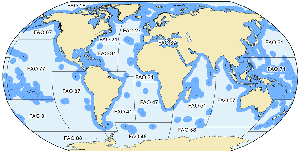
Figure 1. The extent and delimitation of countries’ Exclusive Economic Zones (EEZs), as declared by individual countries, or as defined by the Sea Around Us based on the fundamental principles outlined in UNCLOS (i.e., 200 nautical miles or mid-line rules), and the FAO statistical areas by which global catch statistics are reported. Note that for several FAO areas, some data exist by sub-areas as provided through regional organizations (e.g., ICES for FAO area 27). The Sea Around Us makes use of these spatially refined data to improve the spatial allocation of catch data.

The country-by-country fisheries catch data reconstructions are based on the rational in Pauly (1998), as first implemented by Zeller et al. (2007). The former contribution asserted (i) there is no fishery with ‘no data’ because fisheries, as social activities throw a shadow unto the other sectors of the economy in which they are embedded, and (ii) it is always worse to put a value of ‘zero’ for the catch of a poorly documented fishery than to estimate its catch, even roughly, because subsequent users of one’s statistics will interpret the zeroes as ‘no catches’, rather than ‘catches unknown’.

Zeller et al. (2007) developed a six-step approach for implementing these concepts, as follows:

1. Identification, sourcing and comparison of baseline reported catch times series, i.e., a) FAO (or other international reporting entities) reported landings data by FAO statistical areas, taxon and year; and b) national data series by area, taxon and year;
2. Identification of sectors (e.g., subsistence, recreational), time periods, species, gears etc., not covered by (1), i.e., missing data components. This is conducted via extensive literature searches and consultations with local experts;
3. Sourcing of available alternative information sources on missing data identified in (2), via extensive searches of the literature (peer-reviewed and grey, both online and in hard copies) and consultations with local experts. Information sources include social science studies (anthropology, economics, etc.), reports, colonial archives, data sets and expert knowledge;
4. Development of data ‘anchor points’ in time for each missing data component, and expansion of anchor point data to country-wide catch estimates;
5. Interpolation for time periods between data anchor points, either linearly or assumption-based for commercial fisheries, and generally via per capita (or per-fisher) catch rates for non-commercial sectors; and
6. Estimation of total catch times series, combining reported catches (1) and interpolated, country-wide expanded missing data series (5).

Since these 6 points were originally proposed, a 7^th point has come to the fore which cannot be ignored:

7. Quantifying the uncertainty associated with each reconstruction.

Here, we first expand on each of these seven reconstruction steps (Figure 2), based on the experience accumulated during the decade-long reconstruction process, when completing or guiding the reconstructions:

Step 1: Identification, sourcing and comparison of existing, reported catch times series.

Implicit in this first step is that the spatial entity be identified and named that is to be reported on (e.g., EEZ of Germany in the Baltic Sea).

For most countries, the baseline data are the statistics reported by member countries to FAO. Whenever available, we also use data reported nationally for a first-order comparison with FAO data, which often assist in identifying catches likely taken in areas beyond national jurisdiction, i.e., either in EEZs of other countries or in high seas waters. The reason for this is that many national datasets do not necessarily include catches by national distant-water fleets fishing and/or landing catches elsewhere. As FAO assembles and harmonizes data from various sources, this first-order comparison enabled catches ‘taken elsewhere’ to be identified and separated from truly domestic (national EEZ) fisheries (see Part 4 for the spatial layering of reconstructed datasets).

For some countries, e.g., those resulting from the breakup of the USSR, and Yugoslavia, this involved sourcing data that the now-newly emerged countries would have reported, had these countries already existed independently in 1950. In other words, we treat all countries recognized in 2010 by the international community (or acting like independent entities with regards to fisheries, e.g., the divided island of Cyprus; Ulman et al. 2014) as having existed from 1950-2010. This was necessary, given our emphasis on ‘places’, i.e., on time-series of catches taken from specific ecosystems. This also applies to islands and other territories, many of which were colonies, and which have changed status and borders since 1950.

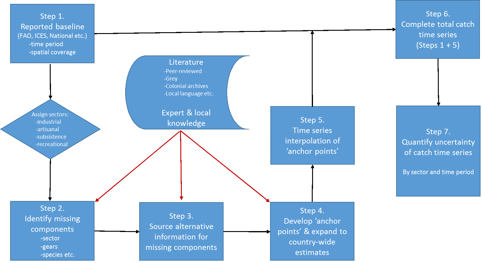
Figure 2. Conceptual representation of the 7-step catch reconstruction approach, as initially described in Zeller et al. (2007) and modified here.

For several countries, the baseline was provided by other international bodies. In the case of countries in Europe, the baseline data generally originated from the International Council for the Exploration of the Sea (ICES), which maintains fisheries statistics by smaller statistical areas, as required given the Common Fisheries Policy of the EU, which largely ignores EEZs. A similar area is the Antarctic continent and surrounding islands, whose fisheries are managed by the Commission for the Conservation of Antarctic Marine Living Resources (CCAMLR), where catches (including discards, a unique feature of CCAMLR) are available by relatively small statistical areas (see e.g., Ainley and Pauly 2013).

When FAO data are used, care is taken to maintain their assignment to different FAO statistical areas for each country (Figure 1). The point here is that, because they are very broad, the FAO statistical areas often distinguish between strongly different ecosystems, for example the Caribbean Sea from the coast of the Eastern Central Pacific in the case of Panama, Costa Rica, Nicaragua, Honduras and Guatemala.

Step 2:  Identification of missing sectors, taxa and gear.

This step is one where the contribution of local co-authors and experts is crucial. Four fisheries sectors potentially occur in the marine fisheries of a given coastal country, with the distinction between large-scale and small-scale being the most important point (Pauly and Charles 2015):

Industrial sector: consisting of relatively large motorized vessels, requiring large sums for their construction, maintenance and operation, either domestically, in the waters of other countries and/or the high seas, and landing a catch that is overwhelmingly sold commercially (as opposed to being consumed and/or given away by the crew). All gears that are dragged or towed across the seafloor or intensively through the water column using engine power (e.g., bottom- and mid-water trawls), no matter the size of the vessel deploying the gear are here considered industrial, following Martín (2012), as are large pirogues (e.g., from Senegal; Belhabib et al. 2014) and ‘baby trawlers’ (in the Philippines; Palomares and Pauly 2014) capable of long-distance fishing, i.e., in the EEZ of neighboring countries. Thus, the industrial sector can also be considered large-scale and commercial in nature;

Artisanal sector: consisting of small-scale (hand lines, gillnets etc.) and fixed gears (weirs, traps, etc.) whose catch is predominantly sold commercially (notwithstanding a small fraction of this catch being consumed or given away by the crew). Thus, our definition of artisanal fisheries relies also on adjacency: they are assumed to operate only in domestic waters (i.e., in their country’s EEZ). Within their EEZ, they are further limited to a coastal area to a maximum of 50 km from the coast or to 200 m depth, whichever comes first. This is the area what we call the Inshore Fishing Area (IFA; see Chuenpagdee et al. 2006). Note that the definition of an IFA assumes the existence of a small-scale fishery, and thus unpopulated islands, although they may have fisheries in their EEZ (which by our definition are industrial), have no IFA. The artisanal sector is thus defined as small-scale and commercial. The other small-scale sectors we recognize are subsistence and recreational fisheries, which overlap in many countries.

Subsistence sector: consisting of fisheries that often are conducted by women and/or non-commercial fishers for consumption by one’s family. However, we also count as subsistence catch the fraction of the catch of mainly artisanal boats that is given away to the crews’ families or the local community (as occurs, e.g., in the Red Sea fisheries; see Tesfamichael et al. 2012). The subsistence sector is thus defined as small-scale and non-commercial.

Recreational sector: consisting of fisheries conducted mainly for pleasure, although a fraction of the catch may end up being sold or consumed by the recreational fishers and their families and friends (Cisneros-Montemayor and Sumaila 2010). Unless data exist on catch-and-release mortalities in a given country, catch from recreational catch-and-release fisheries are not estimated. Often, fisheries that started out as subsistence (e.g., in the 1950s) changed progressively into recreational fisheries as economic development increased in a country and its cash economy grew. The recreational sector is thus defined as small-scale and non-commercial.

Finally, for all countries and territories, we account for two catch types: Landings (i.e., catch that is retained on-board and landed) and discards, which mainly originate from industrial fisheries. Discarded fish and invertebrates are generally assumed to be dead, except for the U.S. fisheries where the fraction of fish and invertebrates reportedly surviving is generally available on a per species basis (McCrea-Strub 2015). Due to a distinct lack of global coverage of information, we do not account for so-called under-water discards, or net-mortality of fishing gears (e.g., Rahikainen et al. 2004). We also do not address mortality caused by ghost-fishing of abandoned or lost fishing gear (Bullimore et al. 2001; He 2006; Renchen et al. 2010), even though it can be substantial, e.g., about 4% of trap-caught crabs worldwide (Poon 2005).

Furthermore, we exclude from consideration all catches of marine mammals, reptiles, corals, sponges and marine plants (the bulk of the plant material is not primarily used for human consumption, but rather for cosmetic or pharmaceutical use). In addition, we do not estimate catches made for the aquarium trade, which can be substantial in some areas in terms of number of individuals, but relatively small in overall tonnage, as most aquarium fish are small or juvenile specimens (Rhyne et al. 2012). Note that at least one regional organization (the Secretariat of the Pacific Community, SPC) is coordinating the tracking of catches and exports of Pacific island countries involved in this trade (see, e.g., Wabnitz and Nahacky 2014). Finally, we do not explicitly address catches destined for the Live Reef Fish Trade (LRFT; see Warren-Rhodes et al. 2003), although, given that these fisheries are often part of normal commercial operations, the catch tonnages of the LRFT is assumed to be addressed in our estimates of commercial catches. Our subsequent estimates of landed value of catches using the global ex-vessel fish price database (see Part 6) will therefore undervalue the catch of any taxa destined directly to the LRFT. All the data omissions indicated above are additional factors why our reconstructed total catches are a conservative metric of the impacts of fishing on the world’s marine ecosystems.

For any country or territory we check whether catches originating from the above fishing sectors are included in the reported baseline of catch data, notably by examining their taxonomic composition, and any metadata, which were particularly detailed in the early decades of the FAO ‘Yearbooks’ (e.g., FAO 1978).

The absence of a taxon known to be caught in a country or territory from the baseline data (e.g., cockles gleaned by women on the shore of an estuary) can also be used to identify a fishery that has been overlooked in the official data collection scheme, as can the absence of reef fishes in the coastal data of a Pacific Island state (Zeller et al. 2015). Note, however, that, to avoid double counting, tuna and other large pelagic fishes, unless known to be caught by a local small-scale fishery (and thus not always reported to a Regional Fisheries Management Organization or RFMO), are not included in this reconstruction step (industrial large pelagic catches are reconstructed using a global approach, see Part 2).

Finally, if gears are identified in national data, but catch data from a gear known to exist in a given country are not included, then it can be assumed that its catch has been missed, as documented by Al-Abdulrazzak and Pauly (2013) for weirs in the Persian Gulf.

Step 3: Sourcing of available alternative information sources for missing data.

The major initial source of information for catch reconstructions is governments’ (and specifically their Department of Fisheries or equivalent agency) websites and publications, both online and in hard copies. Contrary to what could be expected, it is often not the agency responsible for fisheries which supplies the catch statistics to FAO, but other agencies, e.g., some statistical office or agency, with the result that much of the granularity of the original data (i.e., catch by sector, by species or by gear) may be lost even before it reaches Rome. Furthermore, the data request form sent by FAO each year to each country does not explicitly encourage improvements or changes in taxonomic composition, as the form contains the country’s previous years’ data in the same composition as submitted in earlier years, and requests the most recent year’s data. This encourages the pooling of detailed data at the national level into the taxonomic categories inherited through earlier (often decades old) FAO reporting schemes (see e.g., Bermuda, Luckhurst et al. 2003). Thus, by getting back to the original data, much of the original granularity can be regained during reconstructions (e.g., Bermuda reconstruction, Teh et al. 2014). A second major source of information on national catches are international research organizations such as FAO, ICES, or SPC, or a RFMO such as NAFO, or CCAMLR (Cullis-Suzuki and Pauly 2010), or current or past regional fisheries development and/or management projects (many of them launched and supported by FAO), such as the BOBLME Project. All these organizations and projects issue reports and publications describing – sometimes in considerable details – the fisheries of their member countries. Another source of information is obviously the academic literature, now widely accessible through Google Scholar.

A good source of information for the earlier decades (especially the 1950s and 1960s) for countries that formerly were part of colonial empires (especially British or French) are the colonial archives in London (British Colonial Office) and the ‘Archives Nationales d’Outre-Mer’, in Aix-en-Provence, and the publications of O.R.S.TO.M., for the former French colonies. A further good source of information and data are also non-fisheries sources, including household- and/or nutritional-surveys, which can be of great use for estimating unreported subsistence catches. We find the Aquatic Sciences and Fisheries Abstracts (ASFA) and the University of British Columbia library services (and especially its experienced librarians) and its Interlibrary Exchange invaluable for tracking and acquiring such older documents.

Our global network of local collaborators is also crucial in this respect, as they have access to key data sets, publications and local knowledge not available elsewhere, often in languages other than English.

The reconstructions themselves should be consulted for fine-grained information on specific countries or territories, all of which are available online on each EEZ webpage. Every reconstruction we undertake is thoroughly documented and published, either in the peer-reviewed scientific literature, or as detailed technical reports in the publicly accessible and search-engine indexed Fisheries Centre Research Reports series, or the Fisheries Centre Working Paper series, or as reports issued by regional organizations (e.g., BOBLME 2011).

Step 4: Development and expansion of ‘anchor points’.

‘Anchor points’ are catch estimates usually pertaining to a single year and sector, and often to an area not exactly matching the limits of the EEZ or IFA in question. Thus, an anchor point pertaining to a fraction of the coastline of a given country may need to be expanded to the country as a whole, using fisher or population density, or relative IFA or shelf area as raising factor, as appropriate given the local condition. In all cases, we are aware that case studies underlying or providing the anchor point data may had a case-selection bias (e.g., representing an exceptionally good area or community for study, compared to other areas in the same country), and thus we use any raising factors very conservatively. Hence, in many instances, we may actually be underestimating any raised catches.

Step 5: Interpolation for time periods between anchor points.

Fishing, as a social activity involving multiple actors are very difficult to govern; particularly, fishing effort is difficult to reduce, at least in the short term. Thus, if anchor points are available for years separated by multi-year intervals, it will be usually more reasonable to assume that the underlying fishing activity went on in the intervening years with no data. Strangely enough, this ‘continuity’ assumption we take as default is something that some colleagues are reluctant to make, which is the reason why the catches of, e.g., small-scale fisheries monitored intermittingly often have jagged time-series of reported catches. Exceptions to such continuity assumptions are obvious major environmental impacts such a hurricanes or tsunamis (e.g., cyclones Ofa and Val in 1990-1991 in Samoa; Lingard et al. 2012) or major socio-political disturbances, such as military conflicts (e.g., 1989-2003 Liberian civil war; Belhabib et al. 2013), which we explicitly consider with regards to raising factors and the structure of time series. In such cases, our reconstructions mark the event through a temporary change (e.g., decline) in the catch time-series (documented in the text of each catch reconstruction), if only to give pointers for future research on the relationship between fishery catches and natural catastrophes or conflicts. As an aside, we note here that the absence of such a signal in the officially reported catch statistics (e.g., a reduction in catch for a year or two) in countries having experienced a major event of this sort (e.g., Cyclone Nargis in 2008 in Myanmar) is a sure sign that their official catch data are manufactured or at least questionable, without reference to what occurs on the ground (see also Jerven 2013). Overall, our reconstructions assume – when no information to the contrary is available – that commercial catches (i.e., industrial and artisanal) between anchor points can be linearly interpolated, while for non-commercial catches (i.e., subsistence and recreational), we generally use population or number of fishers trends over time to interpolate between anchor points (via per capita rates).

Radical and rapid effort reductions (or even their attempts) as a result of an intentional policy decision (and actual implementation) do not occur widely. One of the few exceptions that comes to mind is the trawl ban of 1980 in Western Indonesia, whose partial implementation is discussed in Pauly and Budimartono (2015). The ban had little or no impact on official Indonesian fisheries statistics for Central and Western Indonesia, another indication that they, also, may have little to do with the realities on the ground

Step 6: Estimation of total catch times series by combining (1) and (5).

A reconstruction is completed when the estimated catch time-series derived through steps 2-5 are combined and harmonized with the reported catch of Step 1. Generally, this will result in an increase of the overall catch, but several cases exist when the reconstructed total catch was lower than the reported catch. The best documented case of this situation is that of mainland China (Watson and Pauly 2001), whose over-reported catches for local waters in the North-west Pacific are inflated by under-reported catches taken by Chinese distant water fleets, which, in the 2000s, operated in the EEZs of over 90 countries, i.e., in most parts of the world’s oceans (Pauly et al. 2014). The step of harmonizing reconstructed catches with the reported baselines obviously goes hand-in-hand with documenting the entire procedure, which is done via a text that is formally published in the scientific literature, or pending publication, is made available online as either a contribution in the Fisheries Centre Research Reports series or as a Fisheries Center Working Paper. These documents (available online via www.seaaroundus.org) should be consulted by anyone intending to work with our data.

Several reconstructions were performed earlier in the mid- to late 2000s, when official data (i.e., FAO statistics or national data) were only available to earlier years. All these cases were subsequently updated to the most recent year of data, either by detailed reconstruction updates or by forward carry procedures (e.g., Zeller et al. 2015) in line with each country’s individual reconstruction approach to estimating missing catch data.

Step 7: Quantifying the uncertainty in (6).

On several occasions, after having submitted reconstructions to peer-reviewed journals, we were surprised by the vehemence with which referees insisted on a quantification of the uncertainty involved in our reconstructions. Our surprise was due to the fact that catch data, in fisheries research, are never associated with a measure of uncertainty, at least not in the form of anything resembling confidence intervals. We pointed out that the issue at hand was not one of precision (i.e., whether, upon re-estimation, we could expect to produce similar results), but about accuracy, i.e., attempting to eliminate a systematic bias, a type of error which statistical theory does not really address. However, this is an ultimately frustrating argument, as is the argument that officially reported catch data, despite being themselves sampled data (e.g., from commercial market sampling, Ulman et al. 2015; or landings site sampling, Jacquet et al. 2010), with unknown but potentially substantial margins of uncertainty, are never expected or thought to require measures of uncertainty.

Hence, we applied to all reconstructions the procedure in Zeller et al. (2015) for quantifying their uncertainly, which is inspired from the ‘pedigrees’ of Funtowicz and Ravetz (1990) and the approach used by the Intergovernmental Panel on Climate Change to quantify the uncertainty in its assessments (Mastrandrea et al. 2010).

Table 1. ‘Scores’ for evaluating the quality of time series of reconstructed catches, with their approximate confidence intervals (IPCC criteria from Figure 1 of Mastrandrea et al. 2010); the percent intervals, here updated from Zeller et al. (2015), are adapted from Ainsworth and Pitcher (2005) and Tesfamichael and Pitcher (2007).
Score		+/- (%)	Corresponding IPCC criteria*
4	Very high	10	High agreement & robust evidence
3	High	20	High agreement & medium evidence or medium agreement & robust evidence
2	Low	30	High agreement & limited evidence or medium agreement & medium evidence or low agreement & robust evidence.
1	Very low	50	Low agreement & low evidence
Mastrandrea et al. (2010) note that “confidence increase” (and hence confidence intervals are reduced) “when there are multiple, consistent independent lines of high-quality evidence”.

This procedure consist of the authors of the reconstructions attributing to each reconstruction a score for each catch estimate by fisheries sector (industrial, artisanal, etc.) in each of three periods (1950-1969, 1970-1989 and 1990-2010) expressing their evaluation of the quality of the time series, i.e., (1) ‘very low’, (2) ‘low’, (3) ‘high’ and (4) ‘very high’. Note the absence of a ‘medium’ score, to avoid the non-choice that this easy option would represent. Each of these scores corresponds to a percent range of uncertainty (Table 1) adapted from Monte-Carlo simulations in Ainsworth and Pitcher (2005) and Tesfamichael and Pitcher (2007). The overall score for the reconstructed total catch of a sector and/or period can then be computed from the mean of the scores for each sectors, weighted by their catch, and similarly for the relative uncertainty. Alternatively, the percent uncertainty for each sector and period can be used for a full Monte Carlo analysis.

Foreign and illegal catches

Foreign catches are catches taken by industrial vessels (by definition, all foreign fishing in the waters of another country is deemed to be industrial in nature) of a coastal state in the EEZ, or EEZ-equivalent waters of another coastal state. As the High Seas legally belong to no one (or to everybody, which is here equivalent), there can be no ‘foreign’ catches in the High Sea. Prior to UNCLOS, and the declaration of EEZs by maritime countries, foreign catches were illegal only if conducted within the territorial waters of such countries (generally, but not always 12 nm). Since the declarations of EEZs by the overwhelming majority of maritime countries, foreign catches are considered illegal if conducted within the (usually 200 nm) EEZ and without access agreement with the coastal state (except in the EU, whose waters are managed by a ‘Common Fisheries Policy’ which implies a multilateral ‘access agreement’).

Such agreements can be tacit and based on historic rights, or more commonly explicit and involving compensatory payment for the coastal state. The Sea Around Us has created a database of such access and agreements, which is used to allocate the catches of distant-water fleets to the waters where they were taken (see Part 4).

Many catch reconstructions, in addition to identifying the catch of domestic fleets, often at least mention the foreign countries fishing in the waters of the country they cover (information we use in our access database), while other reconstructions explicitly quantify these catches (particularly in West Africa, see Belhabib et al. 2012).

This information is then combined and harmonized with:

1. a) the catches deemed to have been taken outside a country’s EEZ, as derived in Step 1 above and further detailed in Part 4, and
2. b) the landings of countries reported by FAO as fishing outside the FAO areas in which they are located (e.g., Spain in FAO Area 27 reporting catches from Area 34, Figure 1), which always identifies these catches as distant-water landings, and thus allows estimation of the catch by foreign fisheries in a given area and even EEZ.

Conservative estimates of discards are then added to these foreign landings, estimated from the discarding rates of the domestic fisheries operating in the countries and/or FAO areas in question.

Catch composition

The taxonomy of catches is what allows catches to be mapped in an ecosystem setting, as different taxa have different distribution ranges and habitat preferences (see Part 3). Also, temporal changes in the relative contribution of different taxa in the catch data also indicate changes in fishing operations and/or in dominance patterns in exploited ecosystems. Thus, various ecosystem state indicators can be derived from catch composition data, e.g., the ‘mean temperature of the catch’ which tracks global warming (Cheung et al. 2013), ‘stock-status plots’ which can provide a first-order assessment of the status of stocks (Kleisner et al. 2013) and the marine trophic index, which reveal instances of “fishing down marine food webs” (Pauly et al. 1998; Pauly and Watson 2005; Kleisner et al. 2014, see also www.fishingdown.org).

Most statistical systems in the word manage to present at least some of their catch in taxonomically disaggregated form (i.e., by species), but many report a large fraction of their catch as over-aggregated, uninformative categories such as ‘other fish’ or ‘miscellaneous marine fishes’ (or ‘marine fishes nei’ [not elsewhere included]). Interestingly, many official national datasets have better taxonomic resolution than the data reported to FAO by national authorities. It is highly likely that this is largely the result of the design of the data request form that FAO distributes to countries each year, which does not actively encourage (nor even suggest) that more detailed national taxonomic resolution data should be provided whenever possible. We have attempted to reduce the contribution of such over-aggregated groups by using taxonomic information from a variety of local and regional studies The species and higher taxa in the catch of a given country or territory can thus belong to either one three groups:

• Species or higher taxa that were already included in the baseline reported data;
• Species or higher taxa into which over-aggregated catches have been subdivided using two or more sets of catch composition data, such that the changing catch composition data reflect at least some of the observed changes of fishing operations and/or in the underlying ecosystem;
• Species or higher taxa into which over-aggregated catches have been subdivided using only one set of catch composition data, and which therefore cannot be expected to reflect changes in catch compositions due to changes in fishing operations and/or changes in the underlying ecosystem. This score is also applied in cases where no local/national information on the taxonomic composition was available, and thus a taxonomic resolution from neighbouring countries was applied.

We have labelled every taxon in the catch time-series of every country with (1), (2) or (3) such that (3) and perhaps also (2) are NOT used to compute indicators such as outlined above (they would falsely suggest an absence of change) – although we fear that this will still occur.

In summary, the approach we developed and utilized for undertaking the catch reconstructions for every maritime country/territory in the world consists of a well-structured system for utilizing all available data sources, and applying a conservative, but comprehensive integration approach.

References

Ainley D and Pauly D (2013) Fishing down the food web of the Antarctic continental shelf and slope. Polar Record 50(1): 92-107.

Ainsworth CH and Pitcher TJ (2005) Estimating illegal, unreported and unregulated catch in British Columbia’s marine fisheries. Fisheries Research 75(1-3): 40-55.

Al-Abdulrazzak D and Pauly D (2013) Managing fisheries from space: Google Earth improves estimates of distant fish catches. ICES Journal of Marine Science 71(3): 450-455.

Ammon U, editor (2001) The dominance of English as a language of science: Effects on other languages and language communities. Walter de Gruyter, Berlin. xiii + 478 p.

Belhabib D, Koutob V, Sall A, Lam V and Pauly D (2014) Fisheries catch misreporting and its implications: The case of Senegal. Fisheries Research 151: 1-11.

Belhabib D, Subah Y, Broh NT, Jueseah AS, Nipey JN, Boeh WY, Copeland D, Zeller D and Pauly D (2013) When ‘reality leaves a lot to the imagination’: Liberian fisheries from 1950 to 2010. Fisheries Centre Working Paper #2013-06, University of British Columbia, Vancouver. 18 p.

Belhabib D, Zeller D, Harper S and Pauly D, editors (2012) Marine fisheries catches in West Africa, 1950-2010, Part I. Fisheries Centre Research Reports 20(3), University of British Columbia, Vancouver. 104 p.

BOBLME (2011) Fisheries catches for the Bay of Bengal Large Marine Ecosystem since 1950. Report prepared by S. Harper, D. O’Meara, S. Booth, D. Zeller and D. Pauly (Sea Around Us Project). Bay of Bengal Large Marine Ecosystem Project, BOBLME-2011-Ecology-16, Phuket. 146 p.

Bullimore BA, Newman PB, Kaiser MJ, Gilbert SE and Lock KM (2001) A study of catches in a fleet of “ghost-fishing” pots. Fishery Bulletin 99(2): 247-253.

Cheung WWL, Watson R and Pauly D (2013) Signature of ocean warming in global fisheries catches. Nature 497: 365-368.

Chuenpagdee R, Liguori L, Palomares MLD and Pauly D (2006) Bottom-up, global estimates of small-scale marine fisheries catches. Fisheries Centre Research Reports 14(8), University of British Columbia, Vancouver. 112 p.

Cisneros-Montemayor AM and Sumaila UR (2010) A global estimate of benefits from ecosystem-based marine recreation: potential impacts and implications for management. Journal of Bioeconomics 12: 245-268.

Cullis-Suzuki S and Pauly D (2010) Failing the high seas: A global evaluation of regional fisheries management organizations. Marine Policy 34(5): 1036-1042.

FAO (1978) Catches and landings (1977). Yearbook of Fishery Statistics Vol. 44, Food and Agriculture Organization, Rome. 343 p.

Funtowicz SO and Ravetz JR, editors (1990) Uncertainty and quality of science for policy. Springer, Kluver, Dortrecht. XI + 231 p.

He P (2006) Gillnets: gear design, fishing performance and conservation challenges. Marine Technology Society Journal 40(3): 12.

Jacquet JL, Fox H, Motta H, Ngusaru A and Zeller D (2010) Few data but many fish: Marine small-scale fisheries catches for Mozambique and Tanzania. African Journal of Marine Science 32(2): 197-206.

Jerven M (2013) Poor numbers: how we are misled by African development statistics and what to do about it. Cornell University Press, Ithaca. 176 p.

Kleisner K, Mansour H and Pauly D (2014) Region-based MTI: resolving geographic expansion in the Marine Trophic Index. Marine Ecology Progress Series 512: 185-199.

Kleisner K, Zeller D, Froese R and Pauly D (2013) Using global catch data for inferences on the world’s marine fisheries. Fish and Fisheries 14(3): 293-311.

Lingard S, Harper S and Zeller D (2012) Reconstructed catches for Samoa 1950-2010. pp. 103-118 In: Harper S, Zylich K, Boonzaier L, Le Manach F, Pauly D and Zeller D (eds.), Fisheries catch reconstructions: Islands, Part III. Fisheries Centre Research Reports 20(5), University of British Columbia, Vancouver.

Luckhurst B, Booth S and Zeller D (2003) Brief history of Bermudian fisheries, and catch comparison between national sources and FAO records. pp. 163-169 In: Zeller D, Booth S, Mohammed E and Pauly D (eds.), From Mexico to Brazil: Central Atlantic fisheries catch trends and ecosystem models. Fisheries Centre Research Reports 11(6), University of British Columbia, Vancouver.

Martín JI (2012) The small-scale coastal fleet in the reform of the common fisheries policy. Directorate-General for internal policies of the Union. Policy Department B: Structural and Cohesion Policies. European Parliament. IP/B/PECH/NT/2012_08, Brussels. Available at www.europarl.europa.eu/studies. 44 p.

Mastrandrea MD, Field CB, Stocker TF, Edenhofer O, Ebi KL, Frame DJ, Held H, Kriegler E, Mach KJ, Matschoss PR, Plattner G-K, Yohe GW and Zwiers FW (2010) Guidance Note for Lead Authors of the IPCC Fifth Assessment Report on Consistent Treatment of Uncertainties. Intergovernmental Panel on Climate Change (IPCC). Available at www.ipcc.ch/pdf/supporting-material/uncertainty-guidance-note.pdf.

McCrea-Strub A (2015) Reconstruction of total catch by U.S. fisheries in the Atlantic and Gulf of Mexico: 1950-2010. Fisheries Centre Working Paper #2015-79, University of British Columbia, Vancouver. 46 p.

Palomares MLD and Pauly D (2014) Reconstructed marine fisheries catches of the Philippines, 1950-2010. pp. 137-146 In: Palomares MLD and Pauly D (eds.), Philippine marine fisheries catches: A bottom-up reconstruction, 1950 to 2010. Fisheries Centre Research Reports 22(1), University of British Columbia, Vancouver.

Pauly D (1998) Rationale for reconstructing catch time series. EC Fisheries Cooperation Bulletin 11(2): 4-10.

Pauly D and Budimartono V, editors (2015) Marine Fisheries Catches of Western, Central and Eastern Indonesia, 1950-2010. Fisheries Centre Working Paper #2015-61, University of British Columbia, Vancouver. 51 p.

Pauly D and Charles T (2015) Counting on small-scale fisheries. Science 347: 242-243.

Pauly D, Belhabib D, Blomeyer R, Cheung WWL, Cisneros-Montemayor A, Copeland D, Harper S, Lam V, Mai Y, Le Manach F, Österblom H, Mok KM, van der Meer L, Sanz A, Shon S, Sumaila UR, Swartz W, Watson R, Zhai Y and Zeller D (2014) China’s distant water fisheries in the 21st century. Fish and Fisheries 15: 474-488.

Pauly D, Christensen V, Dalsgaard J, Froese R and Torres F (1998) Fishing down marine food webs. Science 279: 860-863Pauly D and Charles T (2015) Counting on small-scale fisheries. Science 347: 242-243.

Pauly D and Watson R (2005) Background and interpretation of the ‘Marine Trophic Index’ as a measure of biodiversity. Philosophical Transactions of The Royal Society: Biological Sciences 360: 415-423.

Pikitch EK, Santora C, Babcock EA, Bakun A, Bonfil R, Conover DO, Dayton P, Doukakis P, Fluharty DL, Heneman B, Houde ED, Link J, Livingston PA, Mangel M, McAllister MK, Pope J and Sainsbury KJ (2004) Ecosystem-based Fishery Management. Science 305: 346-347.

Poon AM-Y (2005) Haunted waters: an estimate of ghost-fishing of crabs and lobsters by traps. MSc thesis, University of British Columbia, Fisheries Centre, Vancouver. 138 p.

Renchen GF, Pittman S, Clark R, Caldow C and Olsen D (2010) Assessing the ecological and economic impact of derelict fish traps in the U.S. Virgin Islands. Proceedings of the 63rd Gulf and Caribbean Fisheries Insitute 63: 41-42.

Rhyne AL, Tlusty MF, Schofield PJ, Kaufman L, Morris JA and Bruckner AW (2012) Revealing the Appetite of the Marine Aquarium Fish Trade: The Volume and Biodiversity of Fish Imported into the United States. PloS ONE 7(5): e35808.

Teh L, Zylich K and Zeller D (2014) Preliminary reconstruction of Bermuda’s marine fisheries catches, 1950-2010. Fisheries Centre Working Paper #2014-24, Fisheries Centre, University of British Columbia, Vancouver. 17 p.

Tesfamichael D and Pitcher TJ (2007) Estimating the unreported catch of Eritrean Red Sea fisheries. African Journal of Marine Science 29(1): 55-63.

Tesfamichael D and Pauly D, editors (2012). Catch reconstruction for the Red Sea large marine ecosystem by countries (1950 – 2010). Fisheries Centre Research Reports Vol. 20(1), University of British Columbia, Vancouver. 244 p.

Ulman A, Çiçek B, Salihoglu I, Petrou A, Patsalidou M, Pauly D and Zeller D (2014) Unifying the catch data of a divided island: Cyprus’s marine fisheries catches, 1950-2010. Environment, Development and Sustainability DOI 10.1007/s10668-014-9576-z.

Ulman A, Saad A, Zylich K, Pauly D and Zeller D (2015) Reconstruction of Syria’s fisheries catches from 1950-2010: Signs of overexploitation. Fisheries Centre Working Paper #2015-80, University of British Columbia, Vancouver. 26 p.

Wabnitz C and Nahacky T (2014) Rapid aquarium fish stock assessment and evaluation of industry best practices in Kosrae. Federated States of Micronesia. Secretariat of the Pacific Community, Noumea, New Caledonia. 24 p.

Warren-Rhodes K, Sadovy Y and Cesar H (2003) Marine ecosystem appropriation in the Indo-Pacific: a case study of the live reef fish food trade. Ambio 32(7): 481-488.

Watson R and Pauly D (2001) Systematic distortions in world fisheries catch trends. Nature 414: 534-536.

Zeller D, Booth S, Davis G and Pauly D (2007) Re-estimation of small-scale fishery catches for U.S. flag-associated island areas in the western Pacific: the last 50 years. Fishery Bulletin 105(2): 266-277.

Zeller D, Harper S, Zylich K and Pauly D (2015) Synthesis of under-reported small-scale fisheries catch in Pacific -island waters. Coral Reefs 34(1): 25-39.

2. Reconstructing catches of large pelagic fishes^*

*Cite as: F. Le Manach, A.M. Cisneros-Montemayor, D. Zeller & Daniel Pauly. 2015. Reconstructing catches of large pelagic fishes. In: D. Pauly and D. Zeller (eds). Catch reconstructions: concepts, methods and data sources. Online Publication. Sea Around Us (www.seaaroundus.org). University of British Columbia.

Frédéric Le Manach, Andrés M. Cisneros-Montemayor, Dirk Zeller and Daniel Pauly

Despite tuna fisheries being among the most valuable in the world (FAO 2012), as well as the considerable interest by civil society in the management of large pelagics, there are, to date, no global and comprehensive spatial datasets presenting the historical industrial catches of these species.

Here, we present the methods used to produce a first comprehensive spatial set of large pelagics fisheries catch data.[1] To achieve this, we assembled various existing tuna datasets (Table 1), and harmonized them using a rule-based approach.

For each ocean, the nominal catch data were spatialized according to reported proportions in the spatial data. For example, if France reported 100 tonnes of yellowfin tuna in 1983 using longlines in the nominal dataset, but there were 85 tonnes of yellowfin tuna reported spatially in 1983 by France using longlines, in four separate statistical cells (potentially of varying spatial size), the nominal 100 tonnes for France were split up into those four spatial cells according to their reported proportion of total catch in the spatial dataset. This matching of the nominal and spatial records was done over a series of successive refinements, with the first being the best-case scenario, in which there were matching records for year, country, gear and species. The last refinement was the worst-case scenario, in which there were no matching records except for the year of catch. For example, if France reported 100 tonnes of yellowfin tuna caught in 1983 using longlines, but there were no spatial records for any country catching yellowfin tuna in 1983, the nominal 100 tonnes for France were split up into spatial cells according to their reported proportion of total catch of any species and gear in 1983. After each successive refinement, the matched and non-matched records were stored separately, so that at each new refinement, only the previous step’s non-matched records were used. The matched database was added to at the end of each step. The end result was a catch baseline database containing all matched and spatialized catch records, which sum up to the original nominal catch.

Table 1. Overview of the various data sources used for the creation of global catch maps of industrially caught tuna and other large pelagic fishes.
Ocean	RFMO	Sources		Spatial resolution	Countries/gear/species
		Nominal catch	Spatialized catch
Atlantic	ICCAT	ICCAT website	ICCAT website	1°x1°, 5°x5°, 5°x10°, 10°x10°, 10°x20°, 20°x20°	114/48/142
Indian	IOTC	IOTC website	IOTC website	1°x1°, 5°x5°, 10°x10°, 10°x20°, 20°x20°	57/35/45
Eastern Pacific.	IATTC	IATTC website	FAO Atlas of Tuna and Billfishes	5°x5° c	28/11/19
Western Pacific	WCPFC	WCPFC website	WCPFC website	5°x5°	41/9/9
Southern	CCSBT	Via CCSBT staff	CCSBT website	5°x5°	11/8/1

The catches thus assigned to the various sized tuna-cells (1^o x 1^o to 20^o x 20^o; Table 1) were then spatially allocated to the standard 0.5° x 0.5° degree cells used by the Sea Around Us following the procedure described in Part 4. All artisanal catches (i.e., any gear other than industrial scale longlines, purse-seines, and pole-and-lines,[2] as well as ‘offshore gillnets’) were reallocated to the EEZs of origin of the fleet, as the Sea Around Us defines artisanal fleets as being restricted to domestic areas (Part 1). Here, only the industrial catches are presented.

Finally, a review of the literature was performed for each ocean to collect estimates of discards. Due to the limited amount of country- and fleet-specific data that this search yielded, it was decided that discard percentages should be averaged across the entire time-period and applied to the region of origin of the fleet (e.g., East Asia or Western Europe), rather than the actual country of origin of the fleet. Similarly to the spatialization step described above, successive refinements were then performed to add discards to all reported catch.

Our approach introduces the first harmonized and spatially complete database of global large pelagic fisheries catches, including an estimate of discards. Until now, only regional (RFMO) or globally incomplete (e.g., the FAO Atlas of Tuna and Billfish Catches) databases existed, thus providing a truncated picture of these highly interconnected and global fisheries. The approach sued here, while preliminary in nature, represents the concept and rationale of catch reconstruction as applied to the global large tuna and billfish fisheries. Here, we mention several points that can be improved upon in future iterations:

• The IATTC (Inter-American Tropical Tuna Commission) posed some data problems by not yet releasing the spatialized catches for all gears. We hope that spatialized IATTC data will become available in the future, which will then improve mapping of tuna catches in the northeast Pacific;
• The ICCAT nominal catch database contains some qualitative geographic information (i.e., ‘sub-areas’), which are apparently not geographically defined. Thus, we could not use them to refine our coarse spatialization. If these sub-areas were to become geographically defined, it would allow for improved spatial assignment of catches;
• Discard rates used here only account for a subset of the literature, and difficulties exist in harmonizing them. Feedback from worldwide experts could allow us to refine these rates, by integrating a rule-based approach by gear and country to our discard estimation; and
• Finally, other global databases such as fishbase.org can be used to refine our spatial distribution of the catch by, e.g., restricting species to certain areas of high and consistent occurrence.

References

FAO (2012) The state of world fisheries and aquaculture. Food and Agriculture Organization of the United Nations (FAO), Rome (Italy). 209 p.

FAO (2013) Atlas of Tuna and Billfish Catches. Fishery Statistical Collections [online; updated on June 12, 2013; extracted on June 27, 2013], Food and Agriculture Organization of the United Nations (FAO), Rome (Italy).

Fonteneau A (1997) Atlas of tropical tuna fisheries – World catches and environment. Office de la Recherche Scientifique et Technique Outre-Mer (ORSTOM), Paris (France). 192 p.

Fonteneau A (2009) Atlas of Atlantic Ocean tuna fisheries. IRD Editions, Paris (France). 170 p.

Fonteneau A (2010) Atlas of Indian Ocean tuna fisheries. IRD Editions, Paris (France). 189 p.

IATTC (2013) Resolution C-13-05 – Data confidentiality policy and procedures. 85th meeting of the Inter-American Tropical Tuna Commission, June 10-14, 2013, Veracruz (Mexico). Inter-American Tropical Tuna Commission, La Jolla, CA (USA). 2 p. Available at: http://www.iattc.org/PDFFiles2/Resolutions/C-13-05-Procedures-for-confidential-data.pdf [Accessed: June 16, 2013].

3. Taxon distributions^*

^*Cite as: M.L.D. Palomares, L.D. Tran, A.R. Coghlan, J. Sheedy, W. Cheung, V. Lam & D. Pauly. 2015. Taxon distributions. In: D. Pauly and D. Zeller (eds). Catch reconstructions: concepts, methods and data sources. Online Publication. Sea Around Us (www.seaaroundus.org). University of British Columbia.

Maria-Lourdes.D. Palomares^a, Linh Dinh Tran^c, Amy Rose Coghlan^a, Joseph Sheedy^c, William Cheung^b, Vicky Lam^a and D. Pauly^a

1. ^a) Sea Around Us, University of British Columbia, Vancouver, Canada.
2. ^b) Changing Ocean Unit, University of British Columbia, Vancouver, Canada.
3. ^c) Vulcan Inc., Seattle, Washington, USA.

Ecosystem-based fisheries management (EBFM, Pikitch et al. 2004) must include a sense of place, where fisheries interact with the animals of specific ecosystems. To be useful to researchers, managers and policy makers attempting to implement EBFM schemes, the Sea Around Us presents biodiversity and fisheries data in spatial form onto a grid of about 180,000 half degree latitude and longitude cells which can be regrouped into larger entities, e.g., the Exclusive Economic Zones (EEZs) of maritime countries, or the system of currently 66 Large Marine Ecosystems (LME) initiated by NOAA (Sherman et al. 2007), and now used by practitioners throughout the world.

However, not all the marine biodiversity of the world can be mapped in this manner; thus, while FishBase (www.fishbase.org) includes all marine fishes described so far (more than 15,000 spp.), so little is known about the distribution of the majority of these species that they cannot be mapped in their entirety. The situation is even worse for marine invertebrates, despite huge efforts (see www.sealifebase.org).

     3.1 Scientific and common names

Before taxon distributions can be generated, the taxonomic ‘validity’ of a name needs to be verified, and all names standardized across all data sources being used. The names provided for the taxa included in the Sea Around Us catch data originate either from FAO or from other source material used by catch reconstructions (See Part 1 and Part 2), but were verified using FishBase for fish and SeaLifeBase for non-fish taxa.

Common names, which is what most people know about most organisms, are provided in English, and increasingly also in other languages. FishBase provides common names in other languages for fish, covering nearly 200,000 different names in over 200 languages. FishBase also provides a rationale for the use of common names, and the way the names it contains were assembled.

Scientific names differ in various features, depending on whether they pertain to species, genera, families, orders, classes and phyla

Species names always consist of two parts, a unique genus name (whose first letter is always capitalized) and a species epithet (whose first letter is never capitalized). Both components of the names should be written in italics whenever possible, i.e., Gadus morhua being the scientific species name for the Atlantic cod.

The name of a genus (plural = genera) must be unique (i.e., there is no other such name in the entire animal kingdom) and its first letter is always capitalized. A genus can include one or several species, i.e. Chanos sp., or Stolephorus spp.. For more rules regarding the naming of species and genera, see www.fishbase.de/manual/fishbasespecies_of_fishes.htm

Families consist of one, or more commonly, several genera. Family names among animals always end in -idae, e.g. Gadidae (cods). Family names are not italicized, but always capitalized. Sometimes, ‘common’ names are derived from the scientific names of families, e.g. ‘loliginids’ for squids of the Family Loliginidae, but this usually leads to names that are little used, even when the family was based on a generic name, itself based on a (Latin) common name, e.g., ‘Loligo‘. We have kept such names, however, if they occurred in the FAO catch database, in order to maintain as much compatibility as possible.

Orders consist of one or more families, and their names, in animals, end in -formes. Orders are not italicized but always capitalized. Thus, for example the Gadiformes include the families Gadidae (cods), Merluccidae (hakes), and others, all more closely related to each other than to, e.g., the herrings, sardines, etc. (the Clupeiformes).

Classesconsist of one or more orders, their names in fishes end in ‘-ii’ and in ‘-a’ for invertebrates. Class names are not italicized but always capitalized. Thus, for example both the above mentioned orders Gadiformes and Clupeiformes are in the Class Actinopterygii.

In addition, and to distinguish fish from invertebrates, we also include information on the Phylum of a species. Note that all fishes are under the Phylum Chordata (which is the same taxonomic branch that also includes marine mammals, sea birds, sea snakes, etc., which are not included in the Sea Around Us catch data), while exploited invertebrates generally belong to four phyla, i.e., Arthropoda (lobsters, crabs, shrimps), Mollusca (octopuses, squids, cuttlefishes, bivalves, gastropods). Echinodermata (sea cucumbers, sea stars, sea urchins) and Cnidaria (jellyfishes).

The Sea Around Us data also include broader, but taxonomically ill-defined groups (e.g., ‘miscellaneous marine fishes’, also called ‘marine fishes nei’[3] in FAO parlance), usually the result of suboptimal systems having been set up by various countries for collecting and reporting fisheries catch data. The Sea Around Us strives to disaggregate such data during the reconstruction process, i.e., to allocate them to the appropriate lower taxonomic levels, and we anticipate that the number of broad categories in the database, and especially the amount of catch they represent, will gradually decline.

     3.2 Groups we report on besides ‘taxa’

Because there are more than 2,000 species and almost 1,000 higher taxa included in our global fisheries catches, we have decided to provide taxon specific data on our website for only a user-definable subset of the total number of individual taxa (plus a ‘Others’ group containing all other taxonomic entities combined), but we also provide data using two other types of aggregated groups for all catch.

The first is a general grouping of the catch by 12 broad groups that we call ‘commercial groups’. These are anchovies, herring-like fishes, perch-like fishes, tuna and billfishes, cod-like fishes, salmons and smelts, flatfishes, scorpion fishes, sharks and rays, crustaceans, mollusks, and ‘other fishes and invertebrates’.

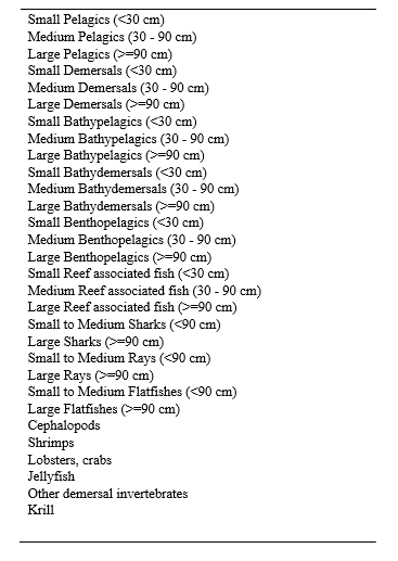
The other grouping is based partly on taxonomy, but mostly on habitat preferences, feeding habits, and maximum size, which define what we call ‘functional groups’ as required for ecosystem modeling (e.g., Ecopath with Ecosim, Christensen et al. 2009). This grouping separates animals by where they live in the water column. Demersal animals that live on or are closely associated with the sea bottom are separated from those that live predominately in the water column or near the water surface (e.g., pelagic). Benthopelagic taxa refer to those that live and feed near the bottom as well as in mid-water or near the surface. Habitat separation is further described by depth zones, with bathypelagic and bathydemersal taxa referring to taxa living in the 1000-4000 m depth zone. Finally, we have separated out reef associated taxa as well as sharks, rays, flatfishes, and a few invertebrate groups (cephalopods, shrimps, lobsters and crabs, jellyfish, krill, and other demersal invertebrates). The functional groups for fishes are further separated by size: small individuals under 30 cm when at maximum length (e.g., small herring species), those that are 30 to 90 cm (e.g. medium sized jacks and mackerels), and those over 90 cm (such as tunas), except for sharks, rays and flatfishes, which are grouped into two categories (small and medium versus large). Overall, we have defined 30 functional groups (Table 1). This grouping system, besides facilitating ecological studies, is useful for studying the impacts of fishing gears, as different functional groups tend to be impacted and targeted by various fishing gears differently.

Table 1. Functional groups as defined by the Sea Around Us for catch reporting and ecosystem modelling.

     3.3 Mapping distributions

We define as ‘commercial’ all marine fish or invertebrate species that are either reported in the catch statistics of at least one of the member countries of the Food and Agriculture Organization of the United Nations (FAO), or are listed as part of commercial and non-commercial catches (retained as well as discarded) in country-specific catch reconstructions (see Part 1 and Part 2). For most species occurring in the landings statistics of FAO, there were enough data in FishBase for at least tentatively mapping their distribution ranges. Similarly, most species of commercial invertebrates had enough information in SeaLifeBase for their approximate distribution ranges to be mapped. We discuss below the procedure we use for taxa that lacked sufficient data for mapping their distribution, which included only few taxa in the FAO statistics, but many from reconstructed catches, including discards.

In the following, we document how such mapping is done. Thus, this contribution presents the methods (improved from Close et al. 2006) by which all commercial species distribution ranges (over 2000 for the 1950-2010 time period) were constructed and/or updated, and consisting of a set of rigorously applied ‘filters’ that will markedly improve the accuracy of the Sea Around Us maps and other products.

The ‘filters’ used here are listed in the order that they are applied. Prior to the ‘filter’ approach presented below, the identity and nomenclature of each species is verified using FishBase or SeaLifeBase, the two authoritative online encyclopedia covering the fishes of the world and marine non-fish animals, respectively, and their scientific and English common names corrected if necessary. This information is then standardized throughout all Sea Around Us databases (see Part 4). Following the creation of all species-level distributions as described here, taxon distributions for higher taxonomic grouping are generated by combining each taxon-level’s contributing components as discussed above and detailed in the section on Creating filters for higher taxa.

Note that the procedures presented here avoid the use of temperature and primary productivity to define or refine distribution ranges for any species, even though these factors strongly shape the distribution of marine fishes and invertebrates (Ekman 1967; Longhurst and Pauly 1987). This was done in order to allow for subsequent analyses of distribution ranges to be legitimately performed using these variables, i.e., to avoid circularity.

Filter 1: FAO Areas

The FAO has divided the world’s oceans into 19 statistical areas for reporting purposes (see Part 1). Information on the occurrence of commercial species within these areas is available primarily through (a) FAO publications and the FAO website (www.fao.org); and (b) FishBase and SeaLifeBase. Figures 1A and 2A illustrate the occurrence by FAO area of Florida pompano (Trachinotus carolinus) and silver hake (Merluccius bilinearis), i.e., examples representing pelagic and demersal species, respectively.

Filter 2: Latitudinal range

The second filter applied in this process is latitudinal ranges. The latitudinal range of a species is defined as the space between its northernmost and southernmost latitudes. This range can be found in FishBase for most fishes and in SeaLifeBase for many invertebrates. For fishes and invertebrates for which this information was lacking, latitudes were inferred from the latitudinal range of the EEZs of countries where they are reported to occur as endemic or native species, and/or from occurrence records in the Ocean Biogeographic Information System website (OBIS; www.iobis.org). Note, however, that recent occurrence records (from the 1980s onwards and known range extensions, e.g., of Lessepsian species) were not used to determine ‘normal’ latitudinal ranges, as they tend to be affected by global warming (Cheung et al. 2009).

A species will not have the same probability of occurrence, or relative abundance throughout its latitudinal range; it can be assumed to be most abundant at the center of its range (McCall 1990). Defining the center of the latitudinal distribution range is done using the following assumptions:

1. For distributions confined to one hemisphere, a symmetrical triangular probability distribution is applied, which estimates the center of the latitudinal range as the average of the range, i.e., [northernmost + southernmost latitude] / 2;
2. For distributions straddling the equator, the range is broken into three parts – the outer two thirds and the inner or middle third. If the equator falls within one of the outer thirds of the latitudinal range, then abundance is assumed to be the same as in (a). If, however, the equator falls in the middle third of the range, then abundance is assumed to be flat in the middle third and decreasing to the poles for the remainder of the range.

Figures 1B and 2B illustrate the result of the FAO and latitudinal filters combined. Both the Florida pompano and the silver hake follow symmetrical triangular distributions as mentioned in (a) above.

Filter 3: Range-limiting polygon

Range-limiting polygons help confine species in areas where they are known to occur, while preventing their occurrence in other areas where they could occur (because of environmental conditions), but do not. There may be one (one water body or restricted occurrence) or set of polygons (several or discontinuous water bodies) which describe the occurrence of a species, the whole compilation of which is here referred to as a distribution extent. Distribution range maps are here defined as published maps which define the geographic range in which a species may occur. Distribution range maps for a vast number of species of commercial fish and invertebrates can be found in various publications, notably FAO’s species catalogues, species identification sheets, guides to the commercial species of various countries or regions, and in online resources, some of which were obtained from model predictions, e.g., Aquamaps (Kaschner et al. 2008; see also www.aquamaps.org). Most range maps are based on observed species occurrences, which may or may not be representative of the actual distribution range of the species.

Occurrence records assume that the observer correctly identified the species being reported, which adds a level of uncertainty to the validity of distribution extents. Most often than not, experts are required to review and validate a component polygon in a distribution extent before it is published, e.g., in FAO or IUCN Red List species fact sheets. This review process is also important, notably for maps that are automatically generated via model predictions such as Aquamaps. Note that for commercially important endemic species, this review process can be skipped as the distribution extent is restricted to the only known habitat and country where such species occurs (generally described by one polygon). In addition, extents for species which were introduced and which have established populations that are important in fisheries, will include both native and introduced ranges (and thus possibly several polygons).

For species without published extents, distribution extents are generated using the filter process described here and compared with the native distribution generated in Aquamaps. Differences between these two ‘model-generated’ maps are verified using data from the scientific literature and OBIS/GBIF (i.e., reported occurrences, notably from scientific surveys). Note that FAO statistics, in which countries report a given species in their catch, can be used as occurrence records, the only exception being if the species was caught by the country’s distant-water fleet.

Polygons are drawn based on the verified map (i.e., with unverified occurrences deleted). Additionally, faunistic work covering the high-latitude end of continents and/or semi-enclosed coastal seas with depauperate faunas (e.g., Hudson Bay, or the Baltic Sea) were used to avoid, where appropriate, distributions reaching into these extreme habitats. The results of this step, i.e., the information gathered from the verification of occurrences, are also provided to FishBase and SeaLifeBase to fill data gaps.

All polygons, whether available from a publication or newly drawn, were digitized with the free software QGIS, and were later used for inferences on equatorial submergence (see below). Figures 1C and 2C illustrate the result of the combination of the first three filters, i.e., FAO, latitude and range-limiting polygons. These parameters and polygons will be revised periodically, as our knowledge of the species in question increases.

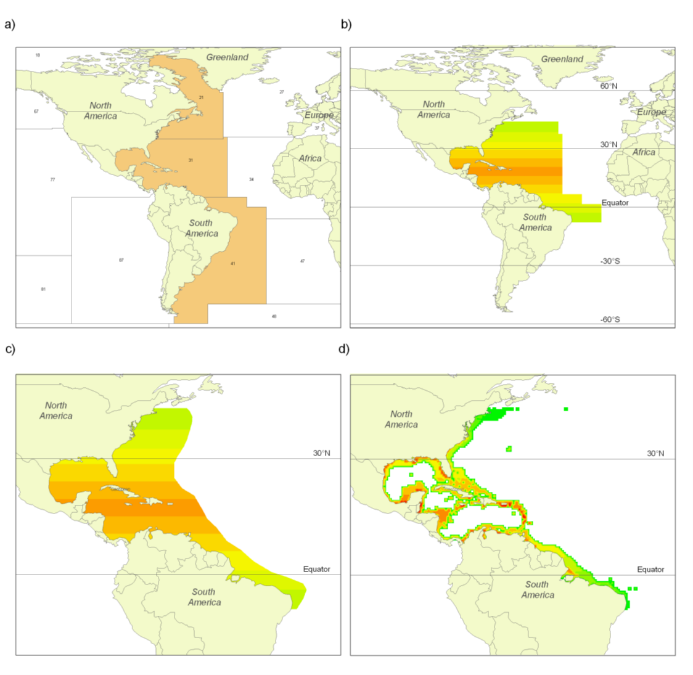
Figure 1. Partial results obtained following the application of the filters used for deriving a species distribution range map for the Florida pompano (Trachinotus carolinus): (A) illustrates the Florida pompano’s presence in FAO areas 21, 31 and 41; (B) illustrates the result of overlaying the latitudinal range (43°N to 9°S; see Smith 1997) over the map in A; (C) shows the result of overlaying the (expert-reviewed) range-limiting polygon over B; and (D) illustrates the relative abundance of the Florida pompano resulting from the application of the depth range, habitat preference and equatorial submergence filters on the map in C.

Figure 2. Partial results obtained following the application of the filters used for deriving a species distribution range map for the silver hake (Merluccius bilinearis): (A) illustrates the silver hake’s presence in FAO areas 21 and 31; (B) illustrates the result of applying the FAO and latitudinal range (55°N to 24°N; see FAO-FIGIS 2001); (C) shows the result of overlaying the (expert-reviewed) range-limiting polygon over B; and (D) illustrates the silver hake’s relative abundance resulting from the application of the depth range, habitat preference and equatorial submergence filters on the map in C.

Note that because this mapping process only deals with commercially-caught species, the distribution ranges for higher level taxa (genera, families, etc.) were generated using the combination of distribution extents from the commercial species level taxa (see section on Creating filters for higher taxa). While this procedure will not produce the true distribution of the genera and families in question, which usually consists of more species than are reported in catch statistics, it is likely that the generic names in the catch statistics refer to the very commercial species that are used to generate the distribution ranges, as these taxa are frequently more abundant than the ones that are not reported in official catch statistics.
 
Filter 4: Depth range

Similar to the latitudinal range, the ‘depth range’, i.e., “[the] depth (in m) reported for juveniles and adults (but not larvae) from the most shallow to the deepest [waters]”, is available from FishBase for most fish species and SeaLifeBase for many commercial invertebrates, along with their common depth, defined as the “[the] depth range (in m) where juveniles and adults are most often found. This range may be calculated as the depth range within which approximately 95% of the species biomass occurs” (Froese et al. 2000). Given this, and based on Alverson et al. (1964), Pauly and Chua (1988), and Zeller and Pauly (2001), among others, the abundance of a species within the water column is assumed to follow a scalene triangular distribution, where maximum abundance occurs at the top one-third of its depth range.

Filter 5: Habitat preference

Habitat preference is an important factor affecting the distribution of marine species. Thus, the aim of this filter is to enhance the prediction of the probability that a species occurs in an area, based on its association with different habitats. Two assumptions are made here:

1. That, other things being equal, the relative abundance of a species in a spatial ½ degree cell is determined by a fraction derived from the number of habitats that a species associates with in that same cell, and by how far the association effect will extend from that habitat; and
2. That the extent of this association is assumed to be a function of a species’ maximum size (maximum length) and habitat ‘versatility’. Thus, a large species that inhabits a wide range of habitats is more likely to occur far from the habitat(s) with which it is associated, while smaller species tend to have low habitat versatility (Kramer and Chapman 1999).

The maximum length and versatility of a species are classified into three categories, and it is assumed that a species can associate with one or more categories with different degrees of membership (0 to 1). A higher membership value means a higher ‘probability’ that the species is associated with that particularly category. The membership values are defined by a pre-specified membership function for each of the length and versatility categories (Figure 3). For example, the striped bass (Morone saxatilis) has a maximum length of 200 cm (total length). Based on the pre-defined membership function presented in Figure 3A, the striped bass has a large body size with a membership of 1. Note that there are maximum length estimates for all the exploited species used by the Sea Around Us, derived from FishBase and SeaLifeBase.

Figure 3. Fuzzy membership functions for the three categories of (A) maximum length and (B) habitat versatility of a species. Habitat versatility is defined as the ratio of the number of habitat types with which a species is associated to the total number of defined habitat types in Table 1. For example, the striped bass (Morone saxatilis) grows to a maximum total length of 200 cm (large body size; degree of membership = 1). It occurs in estuaries and ‘other habitats’ (2 of 5 defined habitats, i.e., versatility = 0.4, low to moderate degree of membership = 0.4-0.6).

The ability of a species to inhabit different habitat types, here referred to as ‘versatility’, is defined as the ratio between the number of habitats with which a species is associated to the total number of habitats as defined in Table 2. These habitats are categorized as ‘biophysical’ (i.e., coral reef, estuary, sea grass, seamount, other habitats), ‘depth-related’ (shelf/slope/abyssal), and ‘distance from coast’ (inshore/offshore). As species are generally specialized towards ‘biophysical’ habitats, this filter only takes those five habitats into consideration. Taking our example again, FishBase lists the following for the striped bass: “Inhabit coastal waters and are commonly found in bays but may enter rivers in the spring to spawn” (Eschmeyer et al. 1983). This associates the striped bass with estuaries and ‘other habitats’ (i.e., when it enters rivers to spawn). Given that the total number of defined biophysical habitats is five, and the striped bass is associated with two of those, then the versatility of striped bass is estimated to be 0.4 (i.e., 2/5). Finally, based on the defined membership functions shown in Figure 3B, the versatility of striped bass is classified as ‘low’ to ‘moderate’, with a membership of approximately 0.4 and 0.6, respectively.

Table 2. Habitat categories used here, and for which global maps are available in the Sea Around Us, with some of the terms typically associated with them (in FishBase, SeaLifeBase and other sources).
Categories	Specifications of global map	Terms often used
Estuary	Alder (2003)	Estuaries, mangroves, river mouth
Coral	UNEP-WCMC (2010)	Coral reef, coral, atoll, reef slope
Sea grass	Not yet available*	Sea grass bed
Seamounts	Kitchingman and Lai (2004)	Seamounts
Other habitats	–	Muddy/sandy/rocky bottom
Continental shelf	NOAA (2004)	Continental shelf, shelf
Continental slope	NOAA (2004)	Continental slope, upper/lower slope
Abyssal	NOAA (2004)	Away from shelf and slope
Inshore	NOAA (2004)	Shore, inshore, coastal, along shoreline
Offshore	NOAA (2004)	Offshore, oceanic
* The Sea Around Us is developing a global map of sea grass, which will be applied when available.

Determining habitat association

Qualitative descriptions relating the commonness (or preference) of a species to particular habitats (as defined in Table 1) are given weighting factors as enumerated in Table 3. Such descriptions are available from FishBase for most fishes and in SeaLifeBase for most commercially important invertebrates. Going back to our example, we thus know that the striped bass occurs in (and thus prefers) brackish water (i.e., estuaries), but enters freshwater (i.e., ‘other habitats’) to spawn. Given the weighting system in Table 3, estuaries is assigned a weight of 0.75 (usually occurs in) and ‘other habitats’ is given a weight of 0.5 (assuming a seasonal spawning period).

Table 3. Common descriptions of relative abundance of species in habitats where they occur and their assigned weighting factors. The weighting factor for ‘other habitats’ is assumed to be 0.1 when no further information is available.
Description	Weightingfactor
Absent/rare	0.00
Occasionally, sometimes	0.25
Often, regularly, seasonally*	0.50
Usually, abundant in, prefer	0.75
Always, mostly, only occurs	1.00
* If a species occurs in a habitat, but no indication of relative abundance is available, a default score of 0.5 is assumed.

Maximum distance of habitat effect

Maximum distance of habitat effect (maximum effective distance) refers to the maximum distance from the nearest perimeter of the habitat which ‘attracts’ a species to a particular habitat. This is defined by the maximum length and habitat versatility of the species using the heuristic rule matrix in Table 4. Taking our example for the striped bass, with a ‘large’ maximum length (membership=1) and ‘low’ to ‘moderate’ versatility (membership values of 0.4 and 0.6), points to a ‘farthest’ maximum effective distance in Table 4. The degree of membership assigned to maximum effective distance is equal to the minimum membership value of the two predicates[4], in this example, 1 vs. 0.4 = 0.4 and 1 vs. 0.6 = 0.6. When the same conclusion is reached from different rules, the final degree of membership equals the average membership value (in this example, (0.4+0.6)/2=0.50).

The maximum effective distance from the associated habitat can be estimated from the ‘centroid value’ of each conclusion category, weighted by the degree of membership. The centroid values for ‘near’, ‘far’ and ‘farthest’ maximum effective distances were defined as 1 km, 50 km and 100 km, respectively. In our example, we obtained membership values of 0.4 for near (1 km) and 0.6 for farthest (100 km) maximum effective distance, respectively. This gives an estimate of (0.4*1 + 0*50 + 0.6*100)/(0.4 + 0 + 0.6) = 60.4 km (see Figure 4).

Table 4. Heuristic rules that define the maximum effective distance from the habitat in which a species occurs. The columns and rules in bold characters represent the predicates (categories of maximum body size and versatility), while those in italics represent the resulting categories of maximum effective distance.
Versatility	Maximum body size
	Small	Medium	Large
Low	Near	Near	Near
Moderate	Far	Far	Farthest
High	Far	Farthest	Farthest

Estimating relative abundance in a spatial cell

Several assumptions are made to simplify the computations. First, it is assumed that the habitat always occurs in the center of a cell and is circular in shape. Second, species density (per unit area) is assumed to be the same across any habitat type; and that density declines linearly from the habitat perimeter to its maximum effective distance. Given these assumptions, the total relative abundance of a species in a cell equals the sum of abundance on and around its associated habitat, expressed as:

B’T = (αj + αj+1 · (1 – αj)) · (1 – A)                          … 4.1)

where B’T is the final abundance, αj is the density away from the habitat from cell j, and A is the habitat area of the cell. The relative abundance resulting from the different habitat types is the sum of relative abundance, and is weighted by their importance to the species.

Although these assumptions on the relationship between maximum length, habitat versatility and maximum distance from the habitat may render uncertain predicted distributions at a fine spatial scale, this routine provides an explicit and consistent way to incorporate habitat considerations into distribution ranges.

Figure 4. Maximum effective distance for striped bass (Morone saxatilis) estimated from the habitat versatility and maximum length of that species (see text).

Filter 6: Equatorial submergence

Ekman (1967) gives the current definition of equatorial submergence: “animals which in higher latitudes live in shallow water seek in more southern regions archibenthal or purely abyssal waters […]. This is a very common phenomenon and has been observed by several earlier investigators. We call it submergence after V. Haecker [1906-1908] who, in his studies on pelagic radiolarian, drew attention to it. In most cases, including those which interest us here, submergence increases towards the lower latitudes and therefore may be called equatorial submergence. Submergence is simply a consequence of the animal’s reaction to temperature. Cold-water animals must seek colder, deeper water layers in regions with warm surface water if they are to inhabit such regions at all.” Equatorial submergence, indeed, is caused by the same physiological constraints which also determine the ‘normal’ latitudinal range of species, as described above, and it shifts due to global warming, i.e., respiratory constraints fish and aquatic invertebrates experience at temperatures higher than that which they have evolved to prefer (Pauly 1998, 2010).

Modifying the distribution ranges to account for equatorial submergence requires accounting for two constraints: (1) data scarcity; and (2) uneven distribution of environmental variables (temperature, light, food, etc.) with depth. FishBase and SeaLifeBase notwithstanding, there is little information on the depth distribution of most commercial species. However, in most cases, the following four data points are available for each species: the shallow end of the depth range (D_shallow), its deep end (D_deep), the poleward limit of the latitudinal range (L_high), and its lower latitude limit (L_low). If it is assumed that equatorial submergence is to occur, then it is logical to also assume that D_shallow corresponds to L_high, and that D_deep corresponds to L_low.

Also, we further mitigate data scarcity by assuming the shape of the function linking latitude and equatorial submergence. Here, two parabolas (P) are used (Figure 5), one for the shallow limits of the depth distribution (P_shallow), and one for the deeper limits (P_deep), with the assumption that both P_shallow and P_deep are symmetrical about the Equator. In addition, maximum depths are assumed not to change poleward of 60⁰ N and 60⁰ S. The uneven distribution of the temperature gradient can be mimicked by constraining P_shallow to be less concave than P_deep by setting the geometric mean (D_gm) of D_shallow and D_deep as the deepest depth that P_shallow can attain. Three points draw the parabolas. In most cases, P_shallow is obtained with D_60°N=0, D_60°S=0 and D_Lhigh=D_shallow, and P_deep with D_60°N=D_gm, D_60°S= D_gm and D_Llow=D_max. If L_high is in the northern hemisphere and L_low is in the south, P_deep is drawn with D_deep at the Equator and conversely for the southern hemisphere. Finally, it is assumed that if a computed P_shallow intercepts zero depth at latitudes higher than 60⁰ N and/or lower than 60⁰ S, then P_shallow is recomputed with D_60°N=D_shallow , D_60°S=D_shallow and D_Lhigh=0.

Figure 5 illustrates three cases of submergence based on different constraints. When this process is applied to a distribution based on latitudinal range and depth, but which did not account for submergence, these have the effect of ‘shaving off’ parts of the shallow-end of that distribution at low latitudes, and similarly, shaving off part of the deep-end end of the distribution at high latitudes. Also, besides leading to narrower and more realistic distribution ranges, this leads to narrowing the temperature ranges inhabited by the species in question, which is important for the estimation of their preferred temperature, as used when modelling global warming effects on marine biodiversity and fisheries.

The key outcome of the process described above consists of distribution ranges such as in Figure 6 for currently over 2,000 taxa, which can be viewed via the Sea Around Us website. They are also accessible via FishBase and SeaLifeBase (click ‘Sea Around Us distributions’ under the ‘Internet sources’ section of the species summary pages). These distribution ranges serve as basis for all spatial catch allocation done by the Sea Around Us (Part 4), and we welcome feedback, i.e., suggested comments or corrections.

Figure 5. Shapes used to generate ‘equatorial submergence’, given different depth/latitude data: (A) Case 1: Barndoor skate (Dipturus laevis) – when the distribution range of the species is at lower latitudes than 60^o N and/or S, the shallow parabola (P_shallow) is assumed to intercept zero at 60^o N and S; (B) Case 2: When a distribution range is spanning the northern and southern hemispheres, as in the case of the Warsaw grouper (Epinephelus nigritus), the deepest depth of the deep parabola (P_deep) is at the Equator; (C) Case 3: Silver hake (Merluccius bilinearis), where the poleward limit of the latitudinal range (L_high) is at higher latitudes than 60^o N and S.

 

Figure 6. ‘Equatorial submergence’ has the effect of ‘shaving off’ areas from the distribution range of the Warsaw grouper, Epinephelus nigritus: (A) Original distribution; (B) Distribution adjusted for ‘equatorial submergence’.

Predictions of distributions from the Sea Around Us algorithm are comparable in performance to other species modeling approaches that are commonly used for marine species (Jones et al. 2012). Specifically, AquaMaps (Kaschner et al. 2008), Maxent (Phillips et al. 2006) and the Sea Around Us algorithm are three approaches that have been applied to predict distributions of marine fishes and invertebrates. Jones et al. (2012) applied these three species distribution modelling methods to commercial fish in the North Sea and North Atlantic using data from FishBase and the Ocean Biogeographic Information System. Comparing test statistics of model predictions with occurrence records suggest that each modelling method produced plausible predictions of range maps for each species. However, the pattern of predicted relative habitat suitability can differ substantially between models (Jones et al. 2013). Incorporation of expert knowledge, as discussed above with reference to Filter 3, generally improves predictions, and therefore was given here particular attention.

Creating filters for higher taxa

The taxonomic hierarchy adapted from FishBase and from SeaLifeBase and described in the section on scientific names, is used here to create a taxon’s‘lineage’ (facilitated by the POSTGRES feature, LTree) to group component species (and we reiterate, only of commercial species included in the Sea Around Us database) by genera, family, order, class and phyla. This basically draws a tree of exploited living resources when visualized. This lineage is the main parameter that enables the ‘roll-up’ (also referred to as a ‘walk’ up or down the tree) to higher taxa of the various filters described in the previous section. Thus for example, the lineage of Atlantic cod (Gadus morhua) is Gadus morhua (species; tree level 6), Gadus (genus; tree level 5), Gadidae (family; tree level 4), Gadiformes (order; tree level 3), Actinopterygii (class; tree level 2), Chordata (phylum; tree level 1).

The latitudinal range, distribution extent, depth range and habitat preference filters for higher taxa were obtained using this roll-up procedure. Latitudinal and depth ranges were rolled-up simply by looking up the minimum and maximum values for component species in a parent taxon’s lineage, i.e., a process that is termed as ‘containment’. Thus, for example, all intermediate values of latitudinal ranges are contained within the northernmost northern range and the southernmost southern range of species in a parent taxon.

Rolling up the habitat index, effective distance and life history parameters for the habitat preference filter differs from the distribution extent procedure. Habitat index, effective distance and the values assigned to each of the habitat filters are treated first; and each habitat filter is treated separately. In cases where there is only one child taxon, the values for this taxon are carried over to the parent taxon. When there are several child taxa, frequency histograms are created in order to obtain a weighted average of the likelihood of occurrence values per habitat filter. Habitat index and effective distance are then calculated using these weighted averages for the parent taxon. Life history parameters, except the VBGF parameter K, for parent taxa are averaged (as arithmetic mean) from the child taxa values. The parameter K is obtained from the average of Linf and Theta Prime and the empirical equation Theta Prime = logK + 2*logLinf (Pauly et al., 1998). This process is repeated for each parent taxon up the tree, using the species level parameters and not the calculated intermediate level parameters.

Rolling up the geographic distribution extent, for example, from species to the genus level, means combining the extents of all the child taxa (here species level) of the immediate parent (here genus level). Thus, the geographic extent of Gadus is built from the extents of the child taxa Gadus morhua, G. macrocephalus and G. ogac in the Sea Around Us database. This procedure is repeated to the highest level taxa. Thus, the extent of Gadidae is built from the extents of the species belonging to 12 gadid genera included in the database. Each child taxon extent is decomposed into its component polygons, which are then arranged in decreasing total area and looped through from largest to smallest area. The geographic extent of, e.g., Gadus, is built when total containment of (or in GIS terminology, the dissolution of) all child taxa polygons is attained. In cases where there is only one child taxon, the extent of this child taxon is carried over to the parent taxon. At the time of writing, there are 2,039 species level taxa in the Sea Around Us catch database (number subject to change over time), which currently belong to 262 genera, 187 families, 19 orders, 11 classes and 5 phyla. Over 82% of the species level taxa have established extents obtained from expert reviewed maps from the IUCN, the FAO and AquaMaps. In cases where there are no available expert reviewed maps, in-depth research of ranges and occurrences are being performed, and the data will be provided to FishBase and SeaLifeBase so that AquaMaps can be generated and thus experts may be called upon to review them. All higher level taxa extents were built through their lineages with commercial species level extents only.

References

Alder J (2003) Putting the coast in the Sea Around Us Project. The Sea Around Us Newsletter, (15): 1-2.

Alverson DL, Pruter AL, Ronholt LL (1964) A Study of Demersal Fishes and Fisheries of the Northeastern Pacific Ocean. Institute of Fisheries, The University of British Columbia, Vancouver.

Cheung WWL, Lam VWY, Sarmiento JL, Kearney K, Watson R and Pauly D (2009) Projecting global marine biodiversity impacts under climate change scenarios. Fish and Fisheries 10: 235-251.

Christensen V, Walters C, Ahrens R, Alder J, Buszowski J, Christensen L, Cheung WL, Dunne J, Froese R, Karpouzi V, Kastner K, Kearney K, Lai S, Lam V, Palomares D, Peters-Mason A, Piroddi C, Sarmiento JL, Steenbeek J, Sumaila RU, Watson R, Zeller D and Pauly D (2009) Database-driven models of the world’s large marine ecosystems. Ecological Modelling 220: 1984-1996.

Close C, Cheung WWL, Hodgson S, Lam VWY, Watson R and Pauly D (2006) Distribution ranges of commercial fishes and invertebrates, p. 27-37 In: M.L.D. Palomares, K.I. Stergiou and D. Pauly (eds.) Fishes in Databases and Ecosystems. Fisheries Centre Research Reports 14(4), University of British Columbia, Vancouver.

Ekman S (1967) Zoogeography of the Sea. Sidgwick & Jackson, London.

Eschmeyer WN, Herald ES and Hammann H (1983) A field guide to Pacific coast fishes of North America. Houghton Mifflin Company, Boston, USA 336 p.

FAO-FIGIS (2001) A world overview of species of interest to fisheries. Chapter: Merluccius bilinearis. Retrieved on 15 June 2005, from www.fao.org/figis/servlet/species?fid=3026. 2p. FIGIS Species Fact Sheets. Species Identification and Data Programme-SIDP, FAO-FIGIS.

Froese R, Capuli E, Garilao C and Pauly D (2000) The SPECIES Table. p. 76-85 In: R. Froese, Pauly, D. (eds.), FishBase 2000: Concept, Design and Data Sources. ICLARM, Los Baños, Laguna, Philippines.

Jones M, Dye S, Pinnegar JK, Warren R and Cheung WWL (2012) Modelling commercial fish distributions: prediction and assessment using different approaches. Ecological Modelling 225:133-145.

Jones MC, Dye SR, Pinnegar JK, Warren R and Cheung WWL (2013) Applying distribution model projections in the present for an uncertain future. Aquatic Conservation: Marine and Freshwater Research 23(5): 710-722.

Kaschner K, Ready JS, Agbayani E, Rius J, Kesner-Reyes K, Eastwood PD, South AB, Kullander SO, Rees T, Close CH, Watson R, Pauly D and Froese R (Editors) (2008) AquaMaps Environmental Dataset: Half-Degree Cells Authority File (HCAF) [see www.aquamaps.org].

Kitchingman A and Lai L (2004) Inferences of potential seamount locations from mid-resolution bathymetric data. p. 7-12 In: T. Morato and D. Pauly (eds.), Seamounts: Biodiversity and Fisheries. Fisheries Centre Research Reports 12(5), University of British Columbia, Vancouver.

Kramer DL and Chapman MR (1999) Implications of fish home range size and relocation for marine reserve function. Environmental Biology of Fishes 55: 65-79.

Longhurst A and Pauly D (1987) Ecology of Tropical Oceans. Academic Press, San Diego, 407 p.

MacCall A (1990) Dynamic Geography of Marine Fish Populations. University of Washington Press, Seattle.

NOAA (2004) ETOPO2 – 2-Minute Gridded Global Relief Data http://www.ngdc.noaa.gov/mgg/fliers/01mgg04.html.

Pauly D (1998) Tropical fishes: patterns and propensities. p. 1-17. In: T.E. Langford, J. Langford and J.E. Thorpe (eds.) Tropical Fish Biology. Journal of Fish Biology 53 (Supplement A).

Pauly D (2010) Gasping Fish and Panting Squids: Oxygen, Temperature and the Growth of Water-Breathing Animals. Excellence in Ecology (22), International Ecology Institute, Oldendorf/Luhe, Germany, xxviii + 216 p.

Pauly D and Chua Thia-Eng (1988) The overfishing of marine resources: socioeconomic background in Southeast Asia. AMBIO: a Journal of the Human Environment 17(3): 200-206.

Pauly, D., J. Moreau and F.C. Gayanilo, Jr. 1998. Auximetric analyses, p. 130-134. In R. Froese and D. Pauly (eds.) FishBase 1998: concepts, design and data sources. ICLARM, Manila, Philippines. 293 p

Phillips SJ, Anderson RP and Schapire RE (2006) Maximum entropy modelling of species geographic distributions. Ecological Modelling 190: 231–259.

Pikitch EK, Santora C, Babcock EA, Bakun A, Bonfil R, Conover DO, Dayton P, Doukakis P, Fluharty DL, Heneman B, Houde ED, Link J, Livingston PA, Mangel M, McAllister MK, Pope J and Sainsbury KJ (2004) Ecosystem-based Fishery Management. Science 305: 346-347.

Sherman K, Aquarone MC and Adams S (2007) Global applications of the Large Marine Ecosystem concept. NOAA Technical Memorandum NMFS NE, 208, 72 p.

Smith CL (1997) National Audubon Society field guide to tropical marine fishes of the Caribbean, the Gulf of Mexico, Florida, the Bahamas, and Bermuda. Alfred A. Knopf, Inc., New York. 720 p.

UNEP-WCMC (2010) Global distribution of coral reefs, compiled from multiple sources. UNEP World Conservation Monitoring Centre. http://data.unep-wcmc.org/datasets/1

Zeller D and Pauly D (2001) Visualisation of standardized life history patterns. Fish and Fisheries 2(4): 344-355.

4. The Sea Around Us databases and their spatial dimensions^*

^*V.W.Y. Lam, A. Tavakolie, D. Pauly & D. Zeller. 2015. The Sea Around Us databases and their spatial dimensions. In: D. Pauly and D. Zeller (eds). Catch reconstructions: concepts, methods and data sources. Online Publication. Sea Around Us (www.seaaroundus.org). University of British Columbia.

Vicky W.Y. Lam, Ar’ash Tavakolie, Daniel Pauly and Dirk Zeller

The individual catch reconstructions for all countries and territories (by EEZ) are all available at www.seaaroundus.org. The underlying taxonomically disaggregated time series of catch data they contain, covering all years since 1950, 4 fishing sectors (industrial, artisanal, subsistence and recreational), 2 catch types (landed versus discarded catch) and 2 types of reporting status (reported versus unreported) for the Exclusive Economic Zones (EEZs) of all maritime countries and territories of the world, or parts thereof, are part of an extensive dedicated database, which interacts with the other databases of the Sea Around Us to generate the spatially allocated fisheries catches for the 180,000 half degree latitude and longitude cells covering the world ocean. These data represent the core product of the Sea Around Us.

     4.1 Catch database

The catch reconstruction database comprises all of the catch reconstruction data by year, fishing country, taxon name, catch amount, fishing sector, catch type, reporting status, input data source and spatial location of catch such as Exclusive Economic Zone (EEZ), FAO area or other area designation (if applicable). The database is further sub-divided into three different data ‘layers’, which include a layer with the catch taken by a fishing country in its own EEZ (called ‘Layer 1’), the catch by each fishing country in other EEZs and/or the high seas (‘Layer 2’), and the catch of all tuna and large pelagic species caught by each fishing country’s industrial fleet (‘Layer 3’). The basic structure of Layers 1 and 2 are identical, while Layer 3 differs slightly in structure due to the nature of the large pelagic input data sets (see Part 2).

Data verification process

The process of data integration into the catch reconstruction database includes a data verification process, which is the first integration step of the original reconstruction dataset and associated reconstruction report. After completing the data verification process for each country dataset, each record is allocated to one of the layers based on the taxon, sector, and the area where the taxon was caught, and is formatted to fit the structure of the final database (see Figure 1 for overview). For example, the total reported landings presented in the reconstruction dataset of each country/territory (which represent the catches landed and deemed reported by national authorities from within the own EEZ of that country/territory) are compared with the reported data as present by FAO on behalf of the respective country/territory for each year. Any ‘surplus’ of FAO data are then considered to have been caught outside the EEZ of the given country/territory, and thus are treated as part of ‘Layer 2’ data. Thus, ‘Layer 2’ data are a derived data product. When any issue with the reconstructed catch data are identified, the issue is raised with the Sea Around Us catch reconstruction team and the original authors of the reconstruction for further checking and refining of the input data. Additional data verification steps include harmonization of scientific taxon names in the reconstruction data with the official, globally recognized and standardized taxon names via the global taxonomic authorities of FishBase (www.fishbase.org) and SeaLifeBase (www.sealifebase.org). Fishing country names and EEZ names are also checked and standardized against the Sea Around Us spatial databases. The fishing country and EEZ names allow us to link the catch data to the foreign fishing access database, which contains the information on which fishing country can access the EEZ of another country (see ‘Foreign fishing access database’ section below).

Figure 1. Data verification process for catch reconstruction data of the Sea Around Us.

     4.2 Foreign fishing access database

The foreign fishing access database, initially derived from the fishing agreement database of FAO (1999), contains observed foreign fishing records, and fishing agreements and treaties that were signed by fishing countries and the host countries in whose EEZs the foreign fleets were allowed to fish. In addition, the database also includes the start and end year of agreements and/or observed access. The type of access is also specified as ‘assumed unilateral’, ‘assumed reciprocal’, ‘unilateral’ or ‘reciprocal’. Also, the type of agreement is recorded in the database and the agreement can be classified into bilateral agreements such as partnership, multilateral agreements such as international conventions or agreements with regional fisheries organizations, private, licensing or exploratory agreements. Additional information contained in this database relates to the type of taxa likely targeted by foreign fleets (e.g., tuna vs. demersal taxa).

This database is used in conjunction with the catch reconstruction database and the taxon distribution database (see Part 3) in the spatial allocation process that assigns catches to the global Sea Around Us ½ x ½ degree latitude and longitude cell system.

     4.3 The Sea Around Us ½ x ½ degree cell system

The Sea Around Us uses a spatial database where the world is divided into a global coverage of 30 arc minute cells (½ x ½ degree). A world cell structure was implemented to conform to the Land-Ocean Interactions in the Coastal Zone (LOICZ) system (www.loicz.org/). Thus, the world is partitioned into 30 x 30 arc minute cells with a top left bounding box corner coordinate at 90°N and 180°W. This results in 180,000 such ½ x ½ degree cells covering the world’s oceans, which form the spatial foundation for all Sea Around Us data.

     4.4 Spatial allocation procedure

The spatial allocation procedure – although it relies on the same global Sea Around Us grid of ½ x ½ degree cells that was used previously – is different from the approach used in the early phase of the Sea Around Us (until 2006) and described in Watson et al. (2004). In the earlier allocations, catches pertaining to large reporting areas (mainly FAO statistical areas) were allocated directly to the half-degree cells, subject only to constraints provided by initially derived taxon distributions for the various taxa (Close et al. 2006), and an earlier and more limited version of the fishing access database granting foreign fleets differential access to the EEZs of various countries (Watson et al. 2004). Thereafter, the catch by a given fishing country in a given EEZ was obtained by summing the catch that had been allocated to the cells making up the EEZ of that country. This process made the spatial allocation overly sensitive to the precise shape and cell-probabilities of the taxon distribution maps, and the precision of very problematic EEZ access rules for different countries. It regularly resulted in sudden and unrealistic shifts of allocated domestic catches into and out of given EEZs purely due to the lifting or imposing of EEZ access constraints. Attempts to improve the allocation procedure with more internal rules made it unwieldy, fragile and extremely time consuming, and thus the Sea Around Us abandoned this approach in the mid-2000s.

The more structured allocation procedure that was devised as a replacement, and is described here (Figure 2), relies on catch data that are spatially pre-assigned (through in-depth catch reconstructions, see Part 1) to the EEZ or EEZ-equivalent waters (for years pre-dating the declaration of individual EEZs) of a given maritime country or territory, and, in the case of small-scale fisheries (i.e., the artisanal, subsistence and recreational sectors), to the Inshore Fishing Areas (Chuenpagdee et al. 2006), and in the case of industrially caught large pelagics, to large ‘tuna cells’ (Part 2). This radically reduces the number of access rules and constraints that the allocation procedure must consider, reduces the chances of fish catches showing up in the EEZs of the wrong country, and dramatically reduces the processing times of the allocation procedure.

Previously, we also used the spatial allocation process to simultaneously disaggregate (i.e., taxonomically improve) uninformative taxonomic groups such as ‘miscellaneous marine fishes’ (FAO term: ‘marine fishes nei’) by relying on taxonomic information in neighboring ½ degree cells. This further added to the complexity of the allocation procedure and increased the difficulty of tracing actual country/taxon/catch entities through the process. This step was also discontinued in the new allocation approach. Instead, our ‘new and improved’ allocation procedure disaggregates the input catch data as part of the country-by-country catch reconstruction process (Part 1), with the associated more transparent taxonomic changes documented in the associated technical report for each reconstruction. Within the catch reconstruction database, we keep track of the quality of the taxonomic disaggregation, such that indicators sensitive to the quality of the disaggregation are not computed from inappropriate data (see ‘Catch composition’ in Part 1).

These pre-allocation data processing modifications allow focusing on the truly spatial elements of the allocation, which are handled through a series of conceptual algorithmic steps. The general algorithm of spatial allocation of catches is harmonized for Layers 1, 2, and 3 (Table 1), which allows for a better software flow, while maintaining the conceptual differences in data layers.

Figure 2. Spatial allocation procedure for catch reconstruction data of the Sea Around Us, resulting in the final ½ x ½ degree allocated cell data.

The spatial allocation of the catch is the process of computing the catch that can be allocated to each ½ degree cell based on the overlap of three main components: 1) the catch data, 2) the fishing access observations/agreements, and 3) the biological taxon distributions (Figure 5.2). The relationship/overlap amongst these components is facilitated by a series of Geographic Information System (GIS) layers, which essentially bind them together.

How each data layer is conceptually unique and how it is handled

In Layer 1, the data come spatially organized by each fishing entity’s EEZ(s). The allocation algorithm allocates the small-scale catches (i.e., artisanal, subsistence, and recreational) only to the cells associated with the Inshore Fishing Area (IFA, Chuenpagdee et al. 2006) of that fishing entity’s EEZ, while industrial catches can be allocated anywhere within that fishing entity’s EEZ(s), as long as they remain compatible with the biological taxon distributions. Fishing access agreements are not applicable to this data layer, as a fishing entity (i.e., country) is always allowed to fish in its own EEZ waters. To represent the historical expansion of industrial fishing since the 1950s in each country’s waters, from more easily accessible areas closer to shore to the full extent of each country’s EEZ, we use the depth adjustment function for domestic industrial catches described in Watson and Morato (2013). This function takes into account that, as domestic industrial catches increase over time, an increasing fraction are being taken progressively further offshore (but within EEZ boundaries).

Table 1. Parameters of the three catch data input layers as used in the spatial allocation to ½ x ½ degree cells of the Sea Around Us.
	Layer 1	Layer 2	Layer 3
Taxa included	All except industrial large pelagics	All except large pelagics	Large pelagics (n =140+)
Spatial scope	Country’s own EEZ	Other EEZs and high seas	Global tuna cells
Sectors	Industrial,Artisanal, Subsistence,Recreational	Industrial	Industrial
Distributions	Biological	Biological	Biological
Fishing access	Automatically granted	Used	Used
Granularity of data	EEZ, IFA1	EEZ, high seas, ICES, CCAMLAR, NAFO, FAO and other areas	Six types of tuna cells: 1×1, 5×5, 5×10, 10×10, 10×20, 20×20 degrees lat. long.
1  Inshore Fishing Area (IFA), defined as the area up to 50 km from shore or 200 m depth, whichever comes first (Chuenpagdee et al. 2006). Note that IFAs are defined only along inhabited coastlines.

In Layer 2, the spatial granularity of the catch data can be by EEZ, high seas, or any other form of regional reporting areas, i.e., ICES, CCAMLR, NAFO, or FAO statistical areas. However, in all cases it excludes the fishing entity (fishing country’s) own EEZ waters (which are treated in Layer 1). In Layer 2, the fishing access observations/agreements are used to compute the areas which allow fishing for a particular fishing entity, year, and taxon. Note that we tread EEZ areas prior to each country’s EEZ declaration year as ‘open access’, meaning no restrictions are applied to other countries being allowed access to these waters. Once this area is computed, it is superimposed on the biological taxon distributions to derive the final Layer 2 catch allocation.

In Layer 3, which only covers industrial large pelagics and their associated bycatch and discards, the input catch data are spatially organized by larger tuna cells which range from 1 x 1 to 20 x 20 degrees (Table 1, see also Part 2). Similar to the region specific areas in Layer 2, these larger cells are intersected with all the EEZ boundaries to create a GIS layer which is suitable for use in the algorithm. Thereafter, the fishing access observations/agreements and taxon distributions are applied to calculate the final Layer 3 catch allocation.

The spatial allocation algorithm consists of 4 main steps:

1. Validating and importing the fishing access observations/agreements database;
2. Validating and importing the catch reconstruction database;
3. Importing the biological taxon distributions; and
4. Computing the catch that can be allocated to each ½ degree cell for each data layer in an iterative process (allowing for verifications and corrections to any of the input parameters).

1. Validating and importing the fishing access observations/agreements database

The fishing access observations/agreements are first verified using several consistency and ‘matching’ tests (Figure 2) and, upon passing, they are imported into the main allocation database. This fishing access information is subsequently used in two different processes: (a) the verification process of the catch data (Layers 1, 2, and 3); and (b) the computing of the areas where a given fishing entity (i.e., country) is allow to fish for a specific year and taxon.

2. Validating and importing the catch reconstruction database

The validating and importing of the catch data is a more complex process than the validating and importing process for the fishing access database. This process involves over 20 different pre-allocation data tests (Figure 2). These tests are designed to make sure that the data are coherent from the standpoint of database logic, and do not contain any accidental errors. These tests range from simple tests like “is the TaxonKey valid?” to more complex tests like “validate if the given fishing entity has the required fishing access observations/agreements to fish in the given marine area”. Every single row of catch data is examined via these tests, and if it passes all tests the data row in question is added to the main allocation database. If it fails any of the tests it is returned to the relevant Sea Around Us data experts for review, often involving the original authors of the catch reconstruction (Figure 2). This iterative process is repeated until all the data rows pass all the pre-allocation tests.

The process of importing the catch reconstruction database includes an important sub-module for harmonizing the marine areas. This module is crucial, as the catch data come in a variety of different spatial reporting areas that are not globally homogenous in GIS definitions (e.g., the EEZ of Albania is one entity, while the EEZ of India, Brazil or the US are subdivided into sub-national areas; the north-east Atlantic uses ICES statistical areas, etc.). To harmonize these marine areas and make them accessible to the core allocation process, any given ½ degree cell is split into its constituent countries EEZs and high seas components. Then, the fishing access observations/agreements are applied to this layer to determine which of these ‘shards’ of ½ degree cells are allowing access to a given fishing entity. Once this is determined, these collections of ‘shards’ are assigned to the given row of catch data, the result is a harmonized view of all the different marine areas. Presently, we have assigned over 12,000 marine areas into their constituent ‘shards’ of ½ degree cells, ranging from EEZs and LMEs, to ICES, CCAMLR, NAFO, and FAO statistical areas. The procedure allows future marine areas to be readily assigned.

3. Importing biological taxon distributions

Importing the biological taxon distributions is a fairly straightforward process. The over 2,000 individual taxon distributions (see Part 3) are generated as individual text files (csv format) containing for each ½ x ½ degree cell the specific taxon’s probability of occurrence. These individual taxon distribution files are compiled into a database table for further use.

4. Computing/allocating the catch to ½ degree cells

Once Steps 1-3 are completed, we perform the computations which yield the final spatial ½ x ½ degree allocation results. The catch of a given data row, TotalCatch, of taxon T is distributed amongst eligible ½ degree cells, Cells 1…n, using the following weighted average formula:

Throughout the allocation process, data parameters besides  year and taxon, such as sector, catch type, reporting status etc. are preserved and carried over into the final allocated database.

The final results of the intense and detailed database preparation and spatial allocation are time series of catches by ½ degree cells that are ecologically reliable (i.e., taxa are caught where they occur, and in relation to their relative abundance) and politically likely (e.g., by fishing country and within EEZ waters to which they have access to).

     4.5 Summarizing allocated data by spatial search regions

While some input data contain spatial designations, such as EEZs or FAO areas (Part 1) or large tuna cells (Part 2), no such spatial pre-designations exist for other spatial search regions we offer, such as LMEs, RFMOs, High Seas etc. in any input data. Thus, data presented for these search areas, or any other custom spatial area, are the result of combining the data from subsets of ½ x ½ degree cells (Part 4) covering the area in question.

REFERENCES

Chuenpagdee R, Liguori L, Palomares MLD and Pauly D (2006) Bottom-up, global estimates of small-scale marine fisheries catches. Fisheries Centre Research Reports 14(8), University of British Columbia, Vancouver. 112 p.

Close C, Cheung WWL, Hodgson S, Lam V, Watson R and Pauly D (2006) Distribution ranges of commercial fishes and invertebrates. pp. 27-37 In; Palomares MLD, Stergiou KI and Pauly D (eds.), Fishes in databases and ecosystems. Fisheries Centre Research Reports 14(4), University of British Columbia, Vancouver.

FAO (1999) FAO Fisheries Agreement Register (FARISIS). Committee on Fisheries, 23^rd Session, 15-19 February 1999. COFI/99/INF.9E. 9 p.

Watson R, Kitchingman A, Gelchu A and Pauly D (2004) Mapping global fisheries: sharpening our focus. Fish and Fisheries 5: 168-177.

Watson R and Morato T (2013) Fishing down the deep: Accounting for within-species changes in depth of fishing. Fisheries Research 140: 63-65.

5. Mapping data

Besides providing our data by selected spatial areas such as by EEZs or LMEs via our website, we also generate spatio-temporal maps presenting the results of our process of assigning catches and related data to ecologically meaningful (via explicit taxon probability distributions, see Section 3) and politically feasible space (via our fishing access database, see Section 4.2). This mapping provides a unique visualization tool to better understand the spatio-temporal development of global fisheries, and is being expanded to incorporate a variety of parameter combinations.

Of note is that the map projection we use is an equal area projection, which, unlike the more commonly used Mercator projection, corrects for the over-emphasis of northern hemisphere land and ocean areas, and thus more realistically represents areas and space across the globe, including in the tropics.

Users of Sea Around Us catch maps and the associated ½ x ½ degree data should be aware that the spatial precision implied by our global use of ½ degree lat./long. cells, which is appropriate for coastal cells, is likely problematic for offshore and High Seas cells. This is due to the catches they contain having been derived from spatially reported catch data provided by Regional Fisheries Management Organizations (RFMOs) in much larger spatial cells (1, 5, 10 or even 20 degree lat./long.). Our subsequent allocation of these data to ½ degree cells within each of the RFMO cells is based on our standard allocation approach, as described in Zeller et al. (2016, Marine Policy 70: 145-152). This allocation is not likely to reflect the precise location of catches being taken from each ½ degree cell within each RFMO cell in each year. Thus, users of these data need to evaluate carefully their use of our spatially allocated data, as the spatial scale at which one analyses these data needs to be driven by the type of question one asks (see Amoroso et al. 2018, Science 361(6404): eaat6713; and Kroodsma et al. 2018, Science361(6404): eaat7789 on appropriate scaling). The Sea Around Us, in collaboration with the Global Fishing Watch, is developing improvements in spatial allocations of catch data that address this and related issues.

We anticipate that this mapping tool will be instrumental in refining and improving data and input parameters over time, and we welcome constructive feedback.

6. The global ex-vessel fish price database^*

^*Cite as: R. Sumaila, L. Teh, D. Zeller & D. Pauly. 2015. The global ex-vessel fish price database. In: D. Pauly and D. Zeller (eds). Catch reconstructions: concepts, methods and data sources. Online Publication. Sea Around Us (www.seaaroundus.org). University of British Columbia.

Rashid Sumaila, Lydia Teh, Dirk Zeller and Daniel Pauly

The database described here provides the ex-vessel price, and when combined with the spatially allocated catches, the landed values of fish caught, by major groupings of species. Besides being economic indicators in their own right, the ex-vessel price and landed value of fish are essential pieces of information needed to help manage fishery resources sustainably to achieve long-term economic and social benefits without depleting the resource base. This is because the financial gains from catch when it is landed is one of the primary motivators for fishers to go fishing. Until the development of the current database, there was no single database available publicly where interested members of the public, researchers and managers can easily find landed values of the world’s major commercial fish catches. The Food and Agriculture Organization of the United Nations (FAO) compiles product and processed fish prices, but not ex-vessel prices, from which landed values are calculated.

Data collection and compilation

Ex-vessel price data for the world’s commercial species were compiled from published sources, and the database was first described by Sumaila et al. (2007), and updated by Swartz et al. (2013). The aim was to add value by taking the data already available but widely scattered to a higher level, one that will permit more policy-relevant ecological and economic analysis of fisheries. We concentrated, in the first instance, on data for the major fishing countries on each continent. In this way, we collected data that covered the major fisheries of the world, while putting in place a database structure that allows continuous inclusion of data for more countries over time.

The database runs from 1950 to the year most recently represented by FAO marine fisheries catches, i.e., from the year the FAO started collecting and compiling global fish catch data. It is worth noting that many analyses of global fisheries begin from this year.

We searched all available sources of ex-vessel price data, including the FAO, the statistics office of the OECD, the European Commission, Fisheries and Oceans Canada, the US National Marine Fisheries Service, Statistics Norway, Southeast Asia Fisheries Development Centre (SEAFDEC) and FAO-Globefish, plus libraries, the web and the published literature. We also worked through our partners from all over the world to help us search for data through on-the-ground data collection efforts.

Filling the data gaps

As would be expected, a substantial portion of the data matrix could not be completed with available data. Therefore, we developed an assignment procedure to help fill the gaps.

As described in Sumaila et al. (2007), the collected data from published sources were used with an interpolation process to ensure that all catch records from our global catch database, regardless of taxon, country, region and year, would have assigned prices. Given that prices for most of the world’s catches were available directly from the price database described above, it was possible to use a structured interpolation process to fill in missing cases using data from similar species, similar countries, etc. The general process of interpolation was one of replacing general prices with more specific ones where they were available. This process assumed that the type of animal (i.e., taxon) was the primary determinant of the price. Following this, in order of importance, were the country fishing and the year when the catches were reported. At each step in the interpolation process, the level of specificity in the documentation was recorded. If a more specific price for a catch record occurred in a subsequent step in the process, then the old price, and its record of specificity, was overwritten with the new price. In this way, all catch records recorded in the global database were matched with the most specific and relevant price recorded in the price database, or weighted averages of these (weighted by their individual specificity) when several prices were available. The original interpolation approach was improved by Swartz et al. (2012), which focused on the computation of annual average international prices for each species group, adjusted to domestic prices using the real exchange rate based on national purchasing power parity. Key advantages of the new approach are that it allows a larger number of reported prices to be used in the price estimation, and accounts for relative price level differences that exist between countries. A measure of the price specificity/applicability is computed for each taxon for which a landed value is presented. These measures are used to guide the priorities in further price data collection efforts.

The database

The primary data in the database are nominal ex-vessel prices as obtained, in most cases by dividing officially reported landed values by landings. Ex-vessel prices and landed values are presented in US$ to allow a uniform basis for comparison. However, the starting point for the data is always local ex-vessel prices in local currency, which are converted into US$ equivalents.

There are two parallel parts to the database, namely, ‘nominal’ and ‘real’ ex-vessel prices and landed values. The ‘real’ numbers were determined by using local consumer price indices (CPI, obtained from the World Bank) to convert local ‘nominal’ ex-vessel prices into ‘real’ ex-vessel prices using the year 2010 as basis. These are then converted into year 2010 US$ equivalents.

References

Sumaila UR, Marsden AD, Watson R and Pauly D (2007) A global ex-vessel fish price database: construction and applications. Journal of Bioeconomics 9: 39-51.

Swartz W, Sumaila UR and Watson R (2013) Global ex-vessel fish price database revisited: A new approach for estimating ‘missing’ prices. Environmental Resource Economics 56: 467-480.

[1] The Food and Agriculture Organization of the United Nations (FAO) has published a global, harmonized atlas, but it includes only the catch of 12 species of tuna and billfishes (i.e., albacore, Atlantic bluefin tuna, Atlantic white marlin, bigeye tuna, black marlin, blue marlin, Pacific bluefin tuna, skipjack tuna, southern bluefin tuna, striped marlin, swordfish, and yellowfin tuna; FAO 2013). This atlas is available at: www.fao.org/figis/geoserver/tunaatlas. For reasons of confidentiality of commercial interests, this dataset entirely lacks longline data for the eastern Pacific area after 1962, managed by the IATTC, although some data for the earlier time-period have been published in aggregated form (Fonteneau 1997). A recent resolution on confidentiality rules may however mean that these spatialized data may become publicly available at some point (IATTC 2013). Fonteneau (1997) has also published a global atlas, but did not estimate discards, nor scaled the spatialized data up to 100% of the nominal catch. Updates were published later, but at regional scales and without the Pacific Ocean (Fonteneau 2009, 2010).

[2] Except when labeled ‘non-mechanized’, ‘coastal’, ‘small’ or such that non-industrial fishing can be inferred.

[3] ‘nei’ stands for ‘not elsewhere included’.

[4]  Predicate logic: a generic term for systems of abstract thought applied in fuzzy logic. In this example, the first-order logic predicate is “IF maximum weight is large”, and the second-order logic predicate is “AND versatility is moderate”. The resulting function, i.e., the conclusion category based on the predefined rules matrix in Table 3, is “THEN maximum effective distance is farthest”.

7. Multinational Footprint Method

Method Link